GetStarted

Starting Point: get started with DDP by following some examples.

This document illustrates how basic aspects of discrete dynamic programming are handled by DDP.

This document uses the HTML details tag ...

So it is best viewed in Safari, Chrome or Opera. In those browsers this material is minimized until you click on the wedge.

details is not supported by Firefox or Explorer as of this writing.

Design and Solve a simple DDP model of searching for a low purchase price.
Simulate Data and Compute the likelihood for the search problem
Re-design the search model with continuous offers and reservation prices.
Where to go next

A simple DDP model of searching for a low purchase price.

Here we set up a very simple sequential choice problem. Then we translate the elements of the model into the terms used in DDP. Then code that implements the model and solves for optimal decision rules is presented. The output generated by DDP is shown.

Files referred to:

niqlow/examples/GetStarted.ox
niqlow/examples/GetStartedMain.ox

To run the program and see results:

oxl GetStartedMain

Steps to Take From Design to Solution

Define the model
Translate the model into DDP terms
Code the model and apply a solution method to it.
Run the code and look at the output

Define The Model

potentially forever

What does N‾ mean?

N‾ ≡ N-1. So, 5‾ = 4. Since counting starts at 0 the larges value is always the number of values minus 1. But putting N-1 everywhere is not elegant.
For more on notation see Notation and Conventions.

$p$

$\{0,1,2,...,N-1\}$

$$Prob(p' = z) = P_p(z) = 1/N, z \in\ \left\{0,...,N-1\right\}.$$

$P_p()$

transition

While searching the person chooses $a$, where $a=1$ means buy at the offered price and $a=0$ means reject and keep searching. The state variable $d$ indicates whether a decision as been made or not. $d=0$ means still searching, and $d=1$ means a price has been accepted. The transition for $d$ today to $d$ next period can written: $$d' = a\quad \Rightarrow\quad P_d(d';a,d) = I\{d'=a\}.$$ And $d=1$ is a terminal value, which means that decision making ends whenever that value is reached. Utility equals realized costs: search costs, $\lambda > 0$, and the price paid if purchased: $$U(a,p,d) = -(1-d)[ \lambda + ap ]$$ Future returns are discounted by $\delta<1$.

The Solution: prices above the value of continued search are rejected.

Translate the model into DDP terms

The notation used here uses DDP's notation for describing a model. Presuming you are starting with this example this notation is shown here to demonstrate how all aspects of DP problems are part of DDP.

The model's clock is stationary, which is a predefined clock type, InfiniteHorzion. The action vector $\alpha$ contains a single binary ActionVariable: $\alpha = (a).$ The offer price is $p$ is an instance (object) of the SimpleJump class.

State Variable Classes

To keep track of all aspects of a state variable, including how it evolves, state variables are objects of a particular class. A class describes both data and methods (functions) that operate on the data. Further, Ox allows for derived classes and virtual methods, which make it possible to build up a library of different kinds of state variables in DDP. Many kinds of state variables that appear in the literature are already coded and available to be included in your model.

$d$

LaggedAction

d=1

$\overline{\Theta}$

Because price offers are IID it can be put into the exogenous state vector $\epsilon$ contains one variable, ε = (p). Since the transition for $d$ depends the current action it is placed in the endogenous state vector $\theta$, which always contains a time variable as well: $\theta = (d t)$.

Why multiple state vectors

To conserve memory and computation, DDP allows the user to put state variables in different vectors that are treated differently. There are actually two other special state vectors not required in this example, $\eta$ and $\gamma$.

t=0

Utility depends on current state variables, actions and parameters:

$U(\alpha,\epsilon,\theta) = U( (a), (p), (d) ) $ = -(1-d)*[ lam + a*p ]

lam

*

objects

$U()$

Code the model in DDP

The full DDP source code is in examples/DDP/GetStarted.ox.

Declare a class derived from Bellman to represent the problem.

 1:   #import "DDP"
 2:   class Search : Bellman {
 3:   		enum{Noff=10}
 4:   		static 	const		decl 	lam = 2.3;
 5:   		static 	     		decl 	p, d, a;
 6:   		static 	Build();
 7:         static  Create();
 8:         static  Run();
 9:   		 	    Utility();	
      }

.h and .ox files

Usually the segment code above would appear in a separate header (.h or .oxh) file, but in the source code for this example it simply appears at the top of the .ox file.

1. Import

The Ox code relies on the DDP package, so import the compiled code and header information for it. See Multiple files in Ox.

2-8. Class Declaration

A user's DP model is represented by a class (or struct). See OOP in Ox. The class name is Search. It is derived from an underlying class, Bellman. The code inside {} declares variables (data members) and functions (method members) that are needed to code the model. Each instance of a Search created while the program executes will represent one point in the state space. Aspects of the model that are shared across points in the state space are stored as static members of the class. Non-static elements are called automatic in Ox, but something is automatic by default unless the tag static appears when it is declared.

More on static and automatic variables

Here is a single class called A with two static members and one automatic member. Then three new instances (objects) of class A are created using the new operator.

class A {
        static decl  a, b;
        decl  c;
}
d = new A();
e = new A();
f = new A();

There are now three versions of A.c in memory but still only two locations A.a and A.b.

A
 A::a
 A::b
d e f
d.c e.c f.c

A A::a A::b
d	e	f
d.c	e.c	f.c

Note that

A::a  ≡  d.a  ≡  e.a  ≡  f.a.
A::b  ≡  d.b  ≡  e.b  ≡  f.b.
d.c !≡ e.c !≡ f.c

However it is referenced, a and b refer to the same place. On the other hand, each instance of A has a distinct c. So there are 5 distinct storage locations, two shared and three specific to the instance of A.

3: The number of offers $N$ is an enumeration, a way of storing integer constants that Ox shares with C.

4: The parameter $\lambda$ is stored as a static constant (its value is fixed at declaration). More powerfully it could be represented as an object of the Parameter class discussed later.

5: Three data members are declared static but variable (their value can change after the object is created). They store the state variables $p$ and $d$ and the action variable $a$.

6: A function associated with an object is called a method. DDP requires two methods.

NB:

DDP uses the name Method for the class of DP solution methods. (Upper and lower case do matter in Ox.) Unfortunately this may cause some confusion. An attempt in these notes will be made to use "solution method" for dynamic programming method and just "method" when using it to refer to a function that belongs to a class.

The methods Run() and Model() are not required, but they help organize the set up and solution of the model. In addition, they are organized to make it easy to build on the basic Search class without having to modify this code (see Get Started With Data).

7: The required method Utility() cannot be static and must have the name and declaration Utility(). It returns the one-period payoff.

Define the required functions for the model

10:	Search::Utility()  {
11:		return -(1-CV(d))*(lam + CV(p)*CV(a));
		}

Utility returns a column of values for feasible actions. It gets the current value of state variables by sending their objects to the CV() function.

Code to set up and solve the model

12:  Search::Create()	{
13:  	Initialize(new Search());
14:     Build();
15:  	CreateSpaces();
    	}
16:  Search::Build() {
17:    	SetClock(InfiniteHorizon);
18:  	SetDelta(0.99);
19:  	Actions(a = new ActionVariable("a",2));
20:  	EndogenousStates(d = new LaggedAction("d",a));
21:  	d->MakeTerminal(1);	
22:    	ExogenousStates(p = new SimpleJump("p",Noff));
      }
23: Search::Run() {
24:    Create();
25:    VISolve();
26:    Delete();
    }

Create the Problem: 13. The user's code must call the Initialize() method before setting up the model.
More on Initialize
Initialize() works only on static elements of the model, and these must be set before any instances of the model are created with new. So it is not possible to put these tasks in the constructor for DP. The user may declare a Initialize() method if they expect the class (Search) to be used as a base for other derived classes. Then Search::Initialize() would call DP::Initialize() and the prefix will be required to resolve the name.
The argument sent to Initialize is an object of the model class. An example of the simplest way to do this is show above: new Search(). This creates an object of the user's model class, in the example Search. Initialize will clone this object for each point in the state space of the model.; 14: Code to set up the model must appear after Initialize() and before the CreateSpaces() method is called. This code is contained in Build(). The code inside the Build function could be inserted at this point. However, following this pattern of defining a Create() and Build() function makes it easier to build on code to extend or change a model without copying or altering existing code.; 15: Once all variables have been defined and added to the model a call to CreateSpaces() will create the action, state, and group spaces. This does not solve the model which is done after the creation step.
Add elements to the model during the Build phase: 17: Every DDP model has a clock. There are several predefined clock types, and the user can create their own if necessary. InfiniteHorizon is an enumeration like Noff in the file above which SetClock() uses to create the right kind of clock.; 18: Every DDP model has a discount factor $\delta$. SetDelta() sets its value, which is constant here but could be set to a variable Parameter..; 19: The action $a$ is an object of the ActionVariable class. It is not an ordinary integer as it might be coded in FORTRAN or C. By making it an object DDP can keep track of all the requirements of having a binary choice in the model without making the user do additional programming. When it is created, the user gives the action a label and says how many different values are feasible for the variable, in this case a.N=2. This happens inside the call to Actions(). DDP must know about the action variables in your model. It cannot peer into the Search class and see that a variable a is there and stores an action variable object. On the other side, action variables cannot insert themselves into your model. The routine Actions() adds the argument(s) sent to it to the model, putting them in the action vector $\alpha$.
Assignments in expressions
The fancy bit is that in Ox, like C and other languages, an assignment expression returns a value. So v=6 stores 6 in v and returns 6 as a result. print(v=6) will print 6. A subtle point that is further explained in other parts of the documentation is that Ox will return a reference to a. So what Actions() stores is a pointer to a not a clone or copy of it.; 20-21: Like the action, the state variables $d$ and $p$ are neither a place to store an integer nor a spot in a vector. State variables are objects of a class. Which class they derived from depends on the kind of state variable it is. But all state variables descend from the base StateVariable class. State variables require more information than action variables to be handled properly. In the model $d$ tracks the choice made in the previous period. This kind of state variable appears in many models so a class for that kind of variable is predefined in DDP: the LaggedAction class. The action that d should track is sent as an argument when a new object of the class is created.
Derived Classes
Actually, this class is a great-great-granddaughter of StateVariable, because it is derived from the LaggedAction class which is derived from Lagged which is derived from Deterministic which is derived from StateVariable. Indeed, d and a are fourth cousins, because states and actions are both derived from an underlying Discrete class.
The method EndogenousStates() adds the arguments sent to it to the $\theta$ vector. Recall that d=1 is a terminal state. DDP must know this so that the value of reaching that state is taken from its utility not iterated on using Bellman's equation. MakeTerminal() is a StateVariable method that can take either an integer or a vector of integer values as its argument. d->MakeTerminal(1) would not work if $d$ had not be assigned a state variable in the previous line.; 22: The state variable $p$ takes on one of p.N different values with equal probability. In DDP this is a SimpleJump state variable. Since its transition does not depend on the current state or actions, DDP can be told this an exogenous state variable, reducing memory and computations.
Create the DP environment: 15: After Build() is complete we return to line 15. All elements have been created and added to the model, the user's code calls CreateSpaces(). CreateSpaces() uses all the information available about elements added to the model to create the state space, the feasible Action sets and many other aspects of the problem. To conserve memory requirements and computational time DDP does not create separate points for the exogenous elements of the state space (here $p$). It treats these separately and attaches values related to the exogenous states to the points in the endogenous state space, $\Theta$.
Solve the Model (and more): The DP model is separate from methods to solve it or use it in some way, including simulation and parameter estimation. Solution methods are derived from the Method class, which itself is derived from the Task class. Tasks are coded to go through the state space and do something at each point.; 25: All those details can be left to DDP by calling the function VISolve(). This routine creates an object of the ValueIteration solution type and calls its Solve() method to compute the solution to Bellman's equation for MyModel. It also calls outAllV() so that a summary of the solution is printed to the screen.; ValueIteration is the most straightforward method for solving a DP model is iteration on Bellman's equation, either until convergence with an infinite horizon or backwards from the final decision period in a finite horizon. Other solution methods could be created as well if more than one method will be used to solve the model (for example, to compare them or one to simulate data and another to use while estimating the model).; Using the VISolve() is convenient for testing and illustrating the code. In most applications the model will be solved repeatedly to estimate parameters, compare solution methods, conduct policy experiments, etc. For more control on output and for repeated use it is better for the user to create the Method object and call its Solve() routine directly. One reason is efficiency. VISolve() creates and destroys the value iteration object each time it is called, which would waste computation if it were called repeated.; 26: The Delete() re-initializes the model to be empty, with no variables or other features defined. This is only important for test code like this when another simple might be created after this one.

Summary

A user DP model is derived from Bellman or another class derived from Bellman. The user code must always call Initialize() for the parent class.
Actions and state variables are instances of predefined classes or user-defined classes. They are added the model using DP methods (functions).
Once all elements of the model have been added the user must call CreateSpaces() to set up the state space and other aspects of the model. The user's code must define a function that returns a new instance of their class which is passed to CreateSpaces(), which will call that function for each point in the state space $\Theta$.
The user must provide a Utility method and a function. This replace the virtual method in Bellman of the same name.
The model is solved by creating an solution object and calling its Solve() function. The VISolve() routine will do all this for you when more control of options and repeated solutions is not needed.

Run the code and see the output

The program that implements the simple search model:

examples/DDP/GetStarted.ox.

The code in GetStarted.ox does not run on its own. Like C, Ox needs to find a single routine called main() which is where execution of the program starts. Often main() is defined in a file on its own. To run the code from there the #include directive can be used to bring other code into the program.

A main() program file to run GetStarted:

examples/DDP/GetStartedMain.ox.

main() does only one thing. It calls Run() which does all the work. Since Run() is static it can be called without referring to an instance of the class previously created with the new operator. There does not have to be an instance of the class for a static variable to exist. In general a user will only call static elements of their model. The DDP code will create instances of the class to represent states and process them internally.

From a command prompt in the examples directory (and assuming niqlow/include is on the include path)

Include Path?

When your program relies on external code through the use of #include or #import then Ox needs to be able to find the code on the machine. Computer languages like Ox are designed to look in different places for code so that you do not have to copy everything to the same folder as your program. The list of places to look for things you include is called the include path. And Ox calls its list OX7Path, which is an system environmental variable (if that helps explain it). You can add a folder, such has \Users\Me\Oxpgms to OX7PATH when you run Ox by doing this:

oxl -i\Users\Me\Oxpgms myprog

If you use OxEdit or some other code editing program then you can set it up so folder(s) are added to the include path automatically so you do not have to type it each type. See Ox Path

oxl GetStartedMain

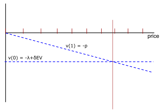
Source: ../examples/output/GetStarted.txt

By default DDP prints out information (you can control the amount by setting DP::Volume). When the spaces are created a summary of the state variables, state spaces, action vectors, and feasible action sets is produced. The Vprint() routine prints out information for each point in the endogenous state space $\Theta$: The value of state variables in $\theta$, $EV(\theta)$, and choice probabilities averaging over the exogenous states. Since EV = -6.26 the searcher will accept any offer with a price below 6.26. There are 7 such offers, 0 through 6, and each is equally likely. So the probability that $a=1$ is 7/10 or 0.7. The rejection probability is 0.3.

Simulate Data and Compute the likelihood for the search problem

DDP knows about data, and it integrates data with solutions of the DP model in different ways. This an example is shown that discusses some of these elements.

A Outcome tracks realizations of a dynamic program including features to account for micro data and maximum likelihood estimation. Unobserved values are accounted for by averaging over their value. a Prediction is like Outcomes except it tracks expected outcomes. It accounts for integrating over probabilities of states and actions. It includes features to account for averaged data and GMM estimation. Auxiliary Values is a mechanism to track things other than states and action. Auxiliary values are defined by the user and added to the model. These are then added to Outcomes and Predictions.

A small example based on simulated data from the simple search model above

This example is based on the Search model described at GetStarted.

Extending the basic MyModel class

Using a derived class the simple search model in GetStarted is extended without touching the existing code or copying it to a new file and modifying. The original code is included (or if it had been split into .h and .ox files, imported), and a new class is derived from the Search class.

struct DerivedSearch : Search {
	static decl u, simdata;
	static Create();
    static Run();
	}

DerivedSearch

Outcome

u

OutcomeDataSet

simdata

Run()

Search

Auxiliary Values

Realized utility is recorded as an AuxiliaryValue. A user may have to define their own new auxiliary value classes, but one of the built-in auxiliary values is RealizedUtility. Here is the code for it, appearing in AuxiliaryValues.h and the source code AuxiliaryValues.ox:

Realize()

$\theta$

$Y$

Since AuxiliaryValue is derived from Quantity it has a current member, v. The job of Realize() is to set v for other aspects of the code to use. In this case, the auxiliary outcome calls Utility() and extracts the element of the vector returned that corresponds to the realized action. By using a virtual method Realize, the base DDP code can update your auxiliary variables for you without knowing ahead of time what those variables are. Also note that an auxiliary value can be sent to CV() after the call to Realize(). For example, here CV(u) will return the realized value of utility of the current outcome. So it is straightforward to build auxiliary variables into econometric objectives, equilibrium conditions, etc. (Besides Realize(), auxiliary values include a virtual Likelihood() method. This is called when computing LogLikelihood().

Modified Run()

DerivedSearch relies on the base Build() routine discussed in GetStarted. All it has to do is create the auxiliary variable and then create a specialized data set object:

DerivedSearch::Create()	{
    Initialize(new DerivedSearch());
	Search::Build();
    u = new RealizedUtility();
	AuxiliaryOutcomes(u);
    CreateSpaces();
	}
DerivedSearch::Run() {
    Create();
    VISolve();
    simdata = new SearchData();

    decl pd = new PanelPrediction();
    pd->Predict(5,TRUE);

    delete simdata, pd;
    Delete;
    }

DataSet Objects

A data set can be simulated or read into DDP using the base OutcomeDataSet class, but it can be convenient to create a derived class to do the work.

struct SearchData : DataSet {
	enum{N=15,MaxOb=20}
    SearchData();
    }

We have stored the size of the simulation we want to run: the enumerated values N and MaxOb will be used in SearchData(). Fifteen searchers will be simulated for up to 20 price draws.

The creator function will do the work.

SearchData::SearchData() {
    OutcomeDataSet("SearchData");
    Volume=LOUD;
	Simulate(15,20,0,TRUE); //TRUE censors terminal states
	Print(1);
	ObservedWithLabel(Search::a,Search::p,Search::d);
	println("Vector of likelihoods when offered price is observed:",exp(EconometricObjective()));
	UnObserved(Search::p);
	println("Vector of likelihoods when offered prices is unobserved:",exp(EconometricObjective()));
    }

SearchData first calls its parent creator method.

The first argument is a name to associate with the data set and the solution method to use during simulation or estimation. Two other arguments can be sent, but in this case they are not needed. In particular, the second argument can be a solution method object so that the dynamic program is solved before the simulation occurs. (In this case, DataSet("Search Data",meth) where member meth was set by the parent Search. However, since Search::Run() is run first and it has already solved the DP model it would be redundant to solve it again.

Simulate() generates the simulated sample by applying the conditional choice probabilities and transitions to initial states.

The simulated panel will consist of N paths of the search model, each of maximum length MaxOb. Since the model has a terminal state, then any path may end before the maximum length. If there were not terminal conditions then the second argument determines how long each path really is. The third argument is a matrix of initial state vectors to use in the simulation. In this case a single state vector is sent. Since the model is stationary (t=0), and the non-absorbing state happens to be d=0, then sending a vector of zeros is appropriate for initial conditions. But in other situations this may not be the desired or well-defined initial state.

The fourth argument being TRUE indicates that when a terminal condition (d=1) is reached that outcome should not be included in the simulated path. The effect is to trim outcomes that are not needed. Once the agent has accepted a price the process is done. So the next state with d=1 is redundant for estimation purposes.

Note: DataSet class does not have a Simulate() method of its own.

Since DataSet is derived from the Panel class the command simdata->Simulate(…) is equivalent to simdata->Panel::Simulate(…). This also means that the user could have made simdata a Panel object instead, if simulation was all that was required, but the data manipulation coming next require a DataSet object.

Print(1) constructs a matrix representation of the data set and prints it to the output screen or log file.

A data set is really a multi-leveled linked list of panels, paths, and outcomes. This makes it possible to write general purpose routines for analyzing the data under various assumptions, such as the likelihood of the panel when some states are unobserved. The object simdata can be printed out to see all this structure, but a great deal of output is produced which is not particularly helpful.

Print process the outcomes into a standard matrix representation.If Print() had been sent a file name with a valid extension then the simulated matrix would have been saved to a file (e.g. such as sim.data or search.xls). Print() calls Flat() to flatten this data structure into a long matrix, one row for each outcome and one column for each element of the full outcome Y* (except for the pointers to other outcomes). Columns for path id and simulated time are added. Flat()is itself a recursive task that builds up the matrix by processing fixed panels, paths and outcomes recursively.

Observability and Masking

ObservedWithLabel(), MatchToColumn() and UnObserved() allow you to control which parts of the outcome is seen in data (and available to econometric methods) and which are missing and require integration over.

By default nothing is observed, so the user must explicitly add variables to the observed list. State variables that are Fixed, are placeholders that take on only one value, so they are implicitly observed. These are marked as force0 so that if reading in from external data the values will be filled in and they do not have to be explicitly observed. ObservedWithLabel() takes one or more action/state/auxiliary objects as arguments. L label of the object is the same as the label or name of the column in the data set, which is how the data is matched with the model variable.

MatchToColumn() takes two arguments. The first is the model variable object. The second is either a label or the index of the column to match the variable with.

Since the code is working with simulated data, the data set already has the full outcome Y* in memory.

When reading in external data, the observability of variables is specified ex ante and then the observable data is read in using Read(const filename). But here, observability is specified ex post.

Masking accounts for unobservability using a fairly complex process (which will be documented more completely in later releases.

Essentially missing observations spawn loops over all possible values when processing the outcome. And the model's probabilistic elements must be used to weight the paths. Further, procedures such as likelihood computation is carried out using backwards recursion not the usual forward recursion. Unless the DataSet Volume is set to SILENT the masking method will print out a table summarizing the observability of the total outcome.

Econometric Objective

DataSet has a virtual method, EconometricObjective(). The default is to compute and return LogLikelihood()

The user can derive their own DataSet class and replace it with an alternative procedure (and other built in objectives, such as GMM, will be provided in later releases). Since it is log-likelihood it is easier to check the exp() in this small example . As with all objectives in FiveO, it returns a vector of values that an algorithm will sum up or use directly to compute Jacobians as needed.

Once data is masked or read in from an external source the value of any variable that was not marked as observed for force0 is now lost even if it were observed originally.

So it is not possible to undo unobservability within a program and a single data set. A second data set can be created without different observability and read in from the same source. (And simulated data could be saved using Print(filename) and read into a new data set.) However, it is possible to undo observability, as the next line illustrates. In the first evaluation of the likelihood the offered price, p was treated as observed. Now, that mark is undone by sending the variable p to UnObserved() and re-masking the data. The next likelihood will integrate out the offered price.

A note on observing the terminal state d.

Since the terminal condition d=1 was censored from the simulated data all the observations have active searchers. However, Mask() does not know this so unless d is marked as unobserved. This creates a problem for rejected offer observations (a=0), because that is feasible when d=1. Thus, the built in log-likelihood will integrate over d=0 and d=1 when offers are rejected unless d is marked as observed. The user should remove d,UseLabel from the observed list and see the implications of this change.

Output

Output produced by running GetStartedData.ox is here:

Source: ../../examples/output/Get_Started_with_data.txt

First, note that the same output is produced as GetStarted.ox, because Search::Run() is called.

Next, the simulation is conducted. Because a Method object was passed to the DataSet the value function was solved again, with the same results.

As requested, the simulated data is printed as a flat matrix.

The column labeled path is an identifier for the realization, and since 10 were requested the ID goes from 0 to 9. Since the probability of accepting an offer is 0.7, most simulated paths will end after one period (t=0). Paths 2 and 7 include rejection of high prices in the first period followed by acceptances in the next period. Also, note that terminating states d=1 are excluded as requested.

The final column of the matrix is the realized utility, which is the auxiliary variable.

The observability of variables is summarized next, in three rows for each aspect of Y*.

The program marked a, p, d as observed. Five aspects of the outcome are fixed (only take on the value 0), so force0 is equal to 1 for them. Since the data are simulated rather than external, each column index is -1.

When EconometricObjective is called the method is used and the model is again solved (in this case unnecessarily because nothing has changed).

The output of the call is a 10x1 vector of log-likelihoods for each IID outcome: that is, each path. The exponent is taken before printing it out in order to get back to a probability (in levels). The fact that each likelihood is exactly 1.0 may be unexpected. But recall, in this simple model there is no continuous shock $\zeta$ and no ex post smoothing of choice probabilities. So the choice probability $P*$ is 1.0 for the optimal choice and 0 otherwise. Since the data are simulated the optimal choice is always chosen, and since p is treated as observed the likelihood conditions on its value.

If external data were read in that included an inconsistent choice (such as rejecting a price of 2), then the likelihood of that observation would be 0.0. (As a modern mathematical language, Ox represents log(0) as -&infty;, and exp(-&infty;) as 0.

Next, the observability of p is undone and the objective is computed again.

The model is resolved, again with the same results and in this case unnecessarily. The new observability is summarized. As noted above, it is not possible to reverse unobservability within a data set, since the observed values are destroyed. But there is no issue with removing p from the observed list and re-masking the data. Now, with prices as treated as unobserved, the model is probabilistic. The model's chance that a=0 is the probability that realized p≥7, or 3/10. The chance of acceptance is 0.7, and for the 8 paths for which the first offer was accepted this is indeed the computed likelihood. This demonstrates that niqlow is able to account for unobservability of states (or actions) based on the model set up and the specified information about outcomes, which are treated independently of the model output and the full outcome Y*.

For the two observations where the first price is rejected the likelihood is 0.21 = 0.7 × 0.3. This demonstrates that a panel of realizations from a single DP is handled properly.

Re-design the search model with continuous offers and reservation prices.

The model is a continuous version of the model above.

Finite time horizon (T=10) to search over job offers
Offers are continuous: $z \sim \Phi(x)$.
Wages not prices: $U = (1-a)\eta + az$
Optimal choice: a reservation wage z* at each t.
That is: policy iteration not value function iteration.

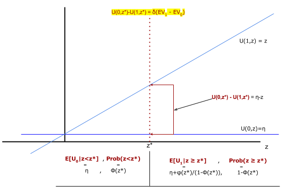
Optimal Behaviour: accept offers above a reservation value z*.
z* solves a non-linear system:

v(1,z*)-v(0,z*)=0

Required Information to solve z*

4 functions of `z*`

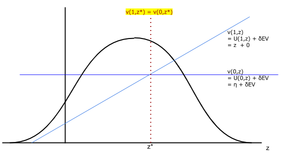
Utility differences at any candidate z*: $U(0,z*)-U(1,z*)$. This information is received by the user-provided method called Uz(z). It returns a column vector with U(0,z*)|U(1,z*)|…. (More generally when there are N choices and N-1 cut-off values it should return a N × N-1 matrix.)

Expected utility for a=0 given z*: $E[U(0,z)|z\le z*]$.

Expected utility for a=1 given z*: $E[U(1,z)|z\gt z*]$.

Probability of acceptable offers: $Prob(z>z*)$

EUtility()

Inputs for solving z*

Code and Output

Header File

Source: examples/misc/WStarA.h

Ox File

Source: examples/misc/WStarA.ox

Output

Source: examples/output/Finite_Horizon.txt

Graph of Reservation values

Source: examples/WstarTestb.pdf

Where to go next

Rust Emet 1987 mle is an example of using external data.

The program /niqlow/examples/main.ox is an interactive program to run examples, test code, and replications. One of the options is to run GetStarted, GetStartedData and GetStartedRValues. To get started with optimization of non-linear objectives, see FiveO/GetStarted.

GetStarted

Summary

A small example based on simulated data from the simple search model above

4 functions of z*

4 functions of `z*`