Read Here
Introduction
Since the early 1980s fields such as macro, labor, and industrial organization have estimated discrete choice, discrete time, dynamic programs. A barrier to empirical DP is the need to write computer code from scratch without benefit of tools tailored to the task. When such computing tools emerge they ease verification, replication and innovation in the area. For example, in applied econometrics, widespread adoption of Stata and R has replaced low-level programming with high-level scripts that are portable and easy to adapt.Why has empirical DP not benefited from development of a similar platform, even as applications and new solutions methods continue to be published? The closest attempt is the Rust (2000) Gauss package available for Rust (1987). There are good reasons to doubt a general platform for empirical DP is feasible. The models are complex, the details vary greatly across fields, and their use involves multiple layers of computation (nested algorithms). Perhaps all they have in common are tools provided by mathematical languages, such as matrix algebra, simulation, and numerical optimization. Matlab packages such as Dynare and VFI Toolkit provide additional tools without offering an integrated platform like Stata.
Does no empirical DP platform exist because it is impossible? If so, why have common platforms emerged in the related areas of non-structural econometrics and dynamic macroeconomics? Or, is it possible, but for some reason a common platform has not emerged from purpose-built code? This paper introduces the software package niqlow to support the latter explanation. The package's design, and how it differs from purpose-built code, suggests why no platform for empirical DP emerged for forty years.
niqlow replaces low-level purpose-built coding with high level tools to design, build and estimate empirical DP models. To demonstrate this claim a simple model is defined and coded with essentially a one-to-one correspondence between the mathematical elements and coding statements. The model is then extended and estimated from data without rewriting code or programming any standard aspects of empirical DP directly.
Starting with Eckstein and Wolpin (1989) and continuing through at least Keane et al. (2011), reviews of the empirical DP literature have attempted to standardize notation with no reference to computing. Because the math does not map directly to code, these frameworks offer limited help to someone developing their own first model. Using niqlow concepts as an intermediate translation between math and working code creates a new way to describe and organize the DP literature. When compared to starting from scratch or "hacking" existing code, new empirical DPs are easier to develop using standardized concepts.
Empirical DP articles contain a standard section that derives the econometric objective step by step. This leaves the impression that the econometrics is specific to the model and the data, which is indeed the case when using purpose-built code. But customized econometric objectives is not a deep feature of other models. For example, a Stata user need not provide a function that returns the log-likelihood for their panel-probit data set. Stata can compute it using details provided by the user. Automation of econometric objectives for empirical DP also emerges in niqlow.
niqlow uses the object-oriented programming (OOP) paradigm to provide menus for state variables, solution methods, and econometric calculations. This paper briefly explains OOP and why it seems fundamental to creating a platform for empirical DP. It also proffers an answer to why such a platform emerged so late compared to other areas of applied economics.
To promote collaborative development, niqlow is open source software housed on github.com under a GPL License. Solution methods can now be compared on different models not simply those chosen by authors proposing a new approach. New solution methods and replications can be added to the platform without recoding.
Ferrall (2021) replicates Rust (1987) in niqlow. Other complete and partial replications are included in the examples section of niqlow. Barber and Ferrall (2021) estimates a lifecycle model of college quality using niqlow.
A Tale of Two Papers
The toolboxes available for empirical work have diverged over time, and this can be traced starting from two early "structural" estimation papers: MaCurdy (1981) and Wolpin (1984). Given resources available at the time, both papers required extensive original programming and significant computational resources.MacCurdy (1981) estimates an approimxated lifecycle labor supply model on panel data. The Lagrange multiplier on a lifecycle budget constraint in the MacCurdy model has a closed form in the estimated specification. That form could have been imposed while estimating other parameters, but it would have to be computed on each iteration of the econometric objective. Instead, MaCurdy (1981) approximates the multiplier as a function of constant characteristics of the person. This approximate model is estimated using two-stage least squares and instrumental variables. Fast-forward to today and MaCurdy's procedure has been reduced to a single line of Stata code:
• xtivreg lnh `xvars' (lnw = exper exper2 L2.wage), first fd
`xvars' is defined elsewhere.)
Wolpin (1984), estimates a lifecyle model of fertility on panel data using maximum likelihood. It defines the approach as a nested solution algorithm that imposes all restrictions of the model on the estimated parameters. Many if not most empirical DP papers follow the same basic strategy. Despite this, nearly all empirical DP models continue to require purpose-built programs for the model. Any change requires re-coding, and certainly no single line in a Stata script solves and estimates a DP model.
Since Wolpin's purpose-built code there has been essentially zero infrastructure developed for empirical DP models. Something has blocked progress in the empirical DP toolbox that did not block IV panel regression code from evolving into single commands in popular packages. Two claims are made here about this roadblock in code development. First, object-oriented programming (OOP) appears essential for removing barriers to a more general economics toolkit. Without shifting to OOP code there was no way to avoid custom coding empirical DP. Second, 6.5 provides an explanation why empirical DP did not shift to OOP until niqlow.
OOP versus PP
Since this paper argues computer programming paradigms have affected the development of economic research, the two relevant paradigms are briefly described here. Readers familiar with OOP can skip this section.Consider the task of creating a computing platform to be used by others to solve their own problems. Call the original coder the programmer and the one using the platform the user. OOP can be compared to the more straightforward procedural programming (PP) approach that has produced most published empirical DP results, in which the programmer and user are essentially the same person or team. Appendix A illustrates the difference between the approaches with the example of coding a package for consumer theory.
A key difference between PP and OOP is how data are stored and processed. In procedural programming (PP) data stored in vectors or other structures are passed to procedures (aka functions or subroutines) to do the work. The procedure sends the results back to the program through a return value or arguments of the procedure. The programmer of a platform would write functions that the user would call in their own program sending their data to the built-in functions.
OOP directly connects (binds) data and the procedures to process them. It does this by putting them together in a class. This brings new syntax and jargon. A class is a template from which objects are created during execution of the program. A class and objects created from it have variables (members) and functions (methods) that process the data stored in the class members.
OOP has three key features that are difficult to code using PP alone. First, a class can be derived from a base class while adding or modifying components. In other words, a class can inherit features from a parent class. The programmer may define child classes from a derived parent to handle different situations the user may confront. Each child in turn might have derived grandchildren. The user can also create their own derived class that inherit only the features of the ancestor classes. Inheritance is a downstream connection between classes created by the programmer for the user.
Second, all objects of the same class can share member data and methods while having their own copies of other members as designed by the programmer. Shared members are sometimes called static because additional storage for them is not created dynamically as objects are created during execution. Static members is a horizontal connection between objects while a program executes.
Third, there is an upstream connection between classes. In OOP jargon this is called a virtual method. Suppose the parent class marks profit() a virtual method. As with all ancestor features, a child class can access profit(). However, the child can define its own method profit(). Since the parent class labels the method virtual it allows the child version to replace the parent version when used by other parent code. That is, the programmer has given the user the option (or the requirement) to inject their own code into the base code. If profit() is not virtual then the user can still create their own version but it will not replace the parent version inside the parent code.
These downstream, horizontal, and upstream connections between data and the functions that process them can be implemented without using objects in procedural programming. No PP platform for empirical DP has been attempted, and no supplemental code has freed users from writing basic functions themselves. This suggests the complex environment of empirical DP requires OOP.
Empirical Dynamic Programming
This section defines key elements of dynamic programming that appear in empirical applications. A simple example is implemented in theniqlow framework before extending it to account for multiple problems and parameter estimation.
A DP Problem
The Primitives
The symbols that define a single generic DP model, in order they are explained in this section, are: $$\th\in\Theta \qquad \al\in A(\th) \qquad P(\thp;\al,\th) \qquad U\l(\al,\th\r) \qquad \delta \qquad \zeta \qquad \psi.$$ The first element is the state $\th$, a vector of state variables: $\th=\pmatrix{s_0 &\dots &s_N}.$ A state is an element of the state space $\Theta.$ Second, at each state an action $\al$ is chosen, a vector of action variables: $\al = \pmatrix{a_0&\dots&a_M}.$ The action is chosen from the feasible choice set $A(\th).$ Third, the next state encountered in the program, denoted $\thp$, follows a semi-Markov transition that depends on the current state and action, $P\l(\thp;\al,\th\r).$When making decisions at $\th$, the agent's objective involves the one-period payoff or utility $U\l(\al,\th\r).$ In niqlow it is treated as a vector-valued function of the feasible action set, so it will be written $U\l(A(\th),\th\r).$ The objective is additive in values of possible states next period discounted by $\delta.$ The values of actions include a shock $\zeta_\al$ contained in the vector $\zeta.$ These shocks often appear in empirical DP to smooth the solution.
Finally, parameters that determine the other primitives are collected in the structural parameter vector $\psi.$ Except for $\Theta$ and $A(\th),$ the other primitives listed above are all possibly implicit functions of $\psi.$ When the empirical DP includes agents solving different problems, exogenous (demographic) data define different problems and they also interact with $\psi.$ The roles of parameters and data are made explicit later.
Bellman's Equation
The value of an action takes the form $$\vvz = U\l(\al,\th\r) + \zeta_\al + \delta E_{\,\al,\th\,}V\l(\thp\r)\label{vv}.$$The final term in the action value \eqref{vv} is the endogenous expected value of future decisions. Optimal state-contingent choices and their value are defined as $$\eqalign{ \al^\star_\zeta(\th) &= {\arg\max}\ \vvz\cr V_\zeta\l(\th\r) &= {\max}_{\ \al \in A(\th)\ }\ \vvz\cr V\l(\th\r) &= \int_{\zeta}\ V_\zeta\l(\th\r) f(\zeta) d\zeta.\cr }\label{V1}$$ Value at $\th$ integrates over optimal value conditional on $\zeta.$ For a model with no $\zeta$ the integral collapses to $V()\equiv V_\zeta().$
The expected value next period sums over the transition of discrete states: $$E_{\,\al,\th\,}V\l(\thp\r) = {\sum}_{\thp\in \Theta}\ V\l(\thp\r)P\st.\label{EV1}$$
Two assumptions about $\zeta$ are built into this expression. First, future shocks are built into $V(\thp)$ which is not affected directly by the current shock because $\zeta$ is IID over time. Second, $\zeta$ can influence the transitions of other state variables only through its effect on $\al.$ These conditions form Rust's (1987) conditional independence (CI) property.
Bellman's equation, also known as the Emax operator, imposes the conditions \eqref{V1} at all states simultaneously: $$\forall\ \th\in\Theta,\quad V(\th) = {\int}_{\zeta}\ \l[ {\max}_{\ \al\in A(\th)\ }\ U\l(\al,\th\r) + \zeta_\al + \delta E_{\,\al,\th\,}V\l(\thp\r)\r]\ f\l(\zeta\r)d\zeta.\label{BE}$$
Conditional Choice Probabilities: Three Flavors
The agent conditions choice on all available information, and $\alpha^\star$ in \eqref{V1} is the set of feasible actions that maximize value at a state. This leads to the first notion of choice probability: from the agent's perspective. In particular, non-optimal choices have 0 probability of occurring. If the optimal choice is unique then the agent chooses it with probability 1. The first flavor of choice probability assigns equal probability to all optimal actions: $$\hbox{CCP1:}\qquad \Pstaraz = { I\left\{ \al\in \al^\star_\zeta(\th) \right\} \over \#\al^\star_\zeta(\th)},\label{CCP1}$$where $I\{\,\}$ is the indicator function and $\#B$ is the cardinality of a set $B.$
The choice probability in \eqref{CCP1} is not continuous in the parameter vector $\psi$ because it includes an indicator function. For example, suppose a small change in a parameter induces a small change in utility. This can shift an action $\al$ from optimal to not optimal and vice versa. $\Pstaraz$ jumps in value which in turn makes an econometric objective built on it discontinuous.
This issue is fixed by treating $\zeta$ as private to the agent. Now choice probabilities based on public information are continuous because they integrate over $\zeta$, leading to the second notion of choice probability: $$\hbox{CCP2:}\qquad\Pstar = \int_{\zeta}\ \Pstaraz f(\zeta) d\zeta.\label{CCP2}$$
For example, when $\zeta$ is extreme value we get the familiar McFadden/Rust form of CCP: $$\Pstar = {e^{\vv}\over {\sum}_{a\in A(\theta)} e^{v(a;\th)}}.\label{CCPEV}$$ The choice probability in \eqref{CCP2} is relevant to the empirical researcher but not to the agent who conditions choice on $\zeta$.
If $\zeta$ is excluded from the model, CCPs may still need to be continuous in the parameter vector $\psi$. This leads to the third notion of conditional choice probability: ex post smoothing using a kernel $K[\ ]$ over all feasible action vectors: $$\hbox{CCP3:}\qquad\Pstarak = K\l[\ v\l(A\l(\th\r);\th\r)\ \r].\label{CCP3}$$
CCP3 adds trembles to CCP1. Equations \eqref{CCP2} and \eqref{CCP3} differ because, in the former, the shocks enter the value function and affect the expected value of future states. In the later, the smoothing takes place separately from the value function. So a logistic kernel is the same functional form as the McFadden/Rust CCP in \eqref{CCPEV}, but the values of the actions are not the same.
The three CCP flavors, un-smoothed as in \eqref{CCP1}, ex-ante smoothed as in \eqref{CCP2}, and ex-post smoothed in \eqref{CCP3}, are all part of niqlow. Within the smoothed classes, the functional or distributional form is a further part of the specification. niqlow provides options for standard functional forms and gives the user the possibility of adding alternatives.
Once solved, the DP model generates an endogenous state-to-state transition: $$P\l(\thp;\th\r) = {\sum}_{\al\in A(\th)}^{} \Pstar P\st.\label{Pqtoq}$$ This transition sums over all feasible actions. Computing \eqref{Pqtoq} is unnecessary in ordinary Bellman iteration, because an agent following the DP will make a choice at each $\th$ they reach. \eqref{Pqtoq} does play a role in predictions and some solution methods discussed later in 5.4.
A final component of a single agent empirical DP model is the set of initial conditions from which data are generated. In non-stationary models it is an exogenous distribution of initial states, $f_0(\th).$ If the environment is stationary then there may be a stationary or ergodic distribution over states, denoted $f_\infty(\th)$ that satisfies $$P\l(\thp;\th\r)f_\infty(\th) = f_\infty(\th).\label{fstar}$$ It is often assumed that data are drawn from the ergodic distribution as the initial condition for estimation or prediction in stationary environments.
Building a DP in niqlow
Empirical DPs have typically been solved using purpose-built programs with hard-coded loops to span the state space $\Theta$ of the model. Different tasks (model solution, prediction or simulation, etc.) use a different nest of loops that must be kept synchronized with the model's assumptions. Introducing another action or state variable requires re-coding and re-synching at the lowest level of the code.
A platform to build and solve any DP model cannot start with this code structure. In particular the hard-coding of the platform by the programmer cannot be model-specific. Instead, the work to build the state space, solve the model, and use it must be constructed from the user's code. The platform must offer standard choices and "plug-and-play" tools for building the model. 1 summarizes how a user would use niqlow following this approach.
niqlow- Declare a new class (template) for the model
- Create the DP
- Initialize: call
Initialize() - Build: add variables and other features to the model
- Create Spaces: call
CreateSpaces() - Code $U()$ and other functions specific to the model.
- Solve: Apply a solution method to compute $V(\th)$ and $\Pstar$
- Use: Simulate data, predict outcomes, estimate parameters, etc.
These steps solve a single agent DP once and use it somehow. Empirical DP almost always requires solving multiple problems multiple times using a nested solution method. In this case the Use and Solve steps above are intertwined (nested). How niqlow handles this is discussed in 6.
None of the steps in 1 include low-level tasks such as: "Code loops to iterate on the value function and check for convergence." These tasks are done for the user based on the high-level elements their code provides. The top-level elements may appear in the code in a different order, but the numbered steps in part B must be executed in that order. Steps B.1 and B.3 each correspond to named functions in niqlow. The amount of coding that other elements in 1 involve depends on the model and its purpose.
Example: Lifecycle Labor Supply
Consider a simple discrete choice lifecycle labor supply model which will be used throughout the rest of the paper to illustrate howniqlow provides a platform for empirical DP. The agent lives 40 periods with the objective of maximizing discounted expected value of working ($m=1$) or not ($m=0$) each period. Earnings $(E)$ come from a Mincer equation that is quadratic in actual experience $M.$ Earnings are subject to a discrete IID shock $e$. Six equations describe the model:
$$\eqalign{
\hbox{Objective:}&\quad E{{\sum}_{t=0}^{39} {0.95}^t} \left[ U\l(m_t ; e_t , M_t\r)+\zeta_m\right] \cr
\hbox{V shocks:}&\quad F(\zeta_m) = e^{e^{-\zeta_m}}\cr
\hbox{Experience:}&\quad M_t = {\sum}_{s=0}^{t-1} m_s;\ M_0 = 0\cr
\hbox{E Shocks:}&\quad e_t \iidsim dZ(15)\cr
\hbox{Earnings:}&\quad E(M,e) = \exp\l\{ \beta_0 + \beta_1 M + \beta_2 M^2 + \beta_3 e \r\} = \exp\l\{ x\beta\r\} \cr
\hbox{Utility:}&\quad U(m;e,M) = mE(M,e) + (1-m)\pi .\cr
}\label{LS1}$$
The earnings shock follows a discretized standard normal distribution taking on $15$ different values, hence the notation $dZ(15).$ The parameter $\pi$ is the utility of not working. The coefficients in the earnings equation are elements of the vector $\beta$ that includes the standard deviation of the earnings shocks, $\beta_3$. An alternative would keep the earnings shock continuous and solve for a reservation value for $m=1.$ This framework and the code to convert the discrete model to the continuous version is described in Appendix C.
The vector $x$ in the earnings function is constructed at each state based on the current values of the state variables. As a bridge to coding \eqref{LS1}, first translate the model into terms used in niqlow.
The Labor Supply Model Using niqlow Concepts
| Element | Value | Category | Params / Notes | |||
|---|---|---|---|---|---|---|
| Clock | $t$ | | Ordinary Aging | T=40. | ||
| CCP | $\zeta$ | ExtremeValue | $\rho=1$. | |||
| Actions | $\al$ | $=$ | $(m)$ | Binary Choice | ||
| States: | $\th$ $\eps$ | $=$ $=$ |
$(M)$ $(e)$ | Action Counter Zvariable | N=40 N=15; $\eps$ defined in 3.6.2. |
|
| Choice Set | $A(\th)$ | $=$ | $\{0,1\}$ | for all $\th$ | ||
| Utility | $U\l(\ \r)$ | $=$ | $\pmatrix{ \pi \cr E(\th)}$ | $E(\th)$ defined in \eqref{LS1}. |
||
This intermediate translation of the math is a new way to summarize the DP literature and a strategy to reduce the fixed cost of building new models. Using these essential elements code can be written corresponding to each step in 1.
A. Declare the template for $\th$
With line numbers added and Ox keywords in bold the code is:
    class LS : ExtremeValue {
1.      static decl m, M, e, beta, pi;
2.             Utility();
3.      static Build();
4.      static Create();
5.      static Earn();
}LS and is derived from the built-in class for extreme value shocks (ExtremeValue). The declaration is not executed. Instead, it is the template for creating each point in the state space while the program executes (step B.2 of the algorithm). Most variables and methods needed by LS are already defined by its ancestor classes. Only details that niqlow cannot know ahead of time need to be added to LS. Line 1 of A declares a member for each element of the model, except $t$ and $\delta,$ which are inherent elements of any problem. All the new members are "static" as briefly explained in 2 as a horizontal connection between objects. An object of the LS class is created for each point in the state space $\Theta,$ but there is only one copy of the static members shared by each object.
Create, Solve and Use
Like C, an Ox program always contains a procedure namedmain() which is where execution begins. LS is designed so that the main procedure is short:
#include "LS.ox"
     main() {
1.        LS::Create();
2.        VISolve();
3.        ComputePredictions();
}Create() method. A user could put all the code inside main() rather than isolating some of it in Create(). Line 2 solves the value function and computes choice probabilities (step C). Solution methods are described in 4. Line 3 generates average values of all the variables based on the solution, as an example of using the solved model (1.D).
B. Create the Model
The three sub-steps in part B are put together inCreate():
    LS::Create() {
1.       Initialize(1.0,new LS());
2.       Build();
3.       CreateSpaces ();
}Build() contains the code specific to the labor supply model. As with main(), Create() could contain more lines of code rather than placing them in Build(). The reason for this becomes apparent when the simple model is extended later on. The version of Initialize() and CreateSpaces() invoked by this code depends on which class LS was derived from.
B.2 Build the Model
In niqlow the action and state vectors are not hard-coded. They are built dynamically as the program executes by adding objects to a list. These tasks must happen in the Build sub-step (1.B2) which here is coded as a separate method:
    LS::Build() {
 1.      SetClock(NormalAging,40);
 2.      m = new BinaryChoice ("m");
 3.      M = new ActionCounter ("M",40,m);
 4.      e = new Zvariable ("e",15);
 5.      Actions (m);
 6.      EndogenousStates (M);
 7.      ExogenousStates (e);
 8.      SetDelta (0.95);
 9.      beta = <1.2 ; 0.09 ; -0.1 ; 0.2>;
10.      pi = 2.0;
}SetClock() to specify the model's clock using one of niqlow's built-in clocks, NormalAging. The parameter for normal aging is the horizon $T,$ here 40 years. If the user wanted to solve an infinite horizon model the code would change the argument to InfiniteHorizon. These choices dictate how storage is created and how Bellman's equation is solved, but from the user's perspective it is simply a different choice of clock.
Line D.2 creates a binary action and stores it in m (declared a member of the LS class in A). Line 5 sends m to Actions() which adds it to the model. The two state variables are created on lines 3 and 4. ActionCounter is a built-in class derived from the base StateVariable class. $M$ needs to know which action variable it is tracking, so $m$ is sent when the counter is created on line 3 along with the number of different values to track (from 0 to 39).
Line 4 creates the earnings shock as object of the Zvariable class. Creating a state variable object does not automatically add it to the model. Lines 6 and 7 do this. Since $e$ is IID it can be placed in the $\eps$ vector by sending it to ExgoenousStates(), explained below. However, $M$ is endogenous because its transition depends on its current value and the action $m.$ It must be placed in $\th$ by sending it to EndogenousStates().
The last three lines of Build() set the value of model parameters. There is no need to formally define the structural parameter vector $\psi$because this version of the model is not estimated. The discount factor $\delta$ is set by calling SetDelta() and is stored internally.
B.3 Creating Spaces
Line 3 C.3 sets up the model by creating the state space, the action spaces and other supporting structures. Selected output from theniqlow function is given in 1. The summary echoes the model's class and its ancestors back to the Bellman class. It echoes the clock type and then list state variables and the number of values they take on. Note that $t$ was added to $\th$ by SetClock(), and it is the second right-most variable in $\th.$ Several state variables are listed that take on 1 value and were not added to the model by the user code. These are placeholder variables for empty vectors explained below. Next, the report lists the size of the state space $\Theta$ and some other spaces. The difference values are discussed later.
CreateSpaces()
0. USER BELLMAN CLASS:    LS | Exteme Value  | Bellman
1. CLOCK:                 3. Normal Finite Horizon Aging
2. STATE VARIABLES
              |eps   |eta |theta -clock        |gamma
                e    s21      M      t     t''     r      f
       s.N     15      1     40     40      1      1      1
3. SIZE OF SPACES
                       Number of Points
    Exogenous(Epsilon)               15
    Endogenous(Theta)                40
    Times                            40
    EV()Iterating                    40
    ChoiceProb.track               1600
    Total Untrimmed               24000
5. TRIMMING AND SUBSAMPLING OF THE ENDOGENOUS STATE SPACE
                           N
    TotalReachable       820
         Terminal          0
     Approximated          0
C. Code Utility and Other Functions
1.C says to code utility and other functions. Utility is not involved in creating the state space so is only called once a solution method begins. The user's utility replaces a virtual utility called insideniqlow algorithms. There are several other virtual methods that the user might need to replace, and some examples appear below.
To match the model specification in \eqref{LS1}, and in anticipation of empirical applications, earnings and utility are coded as separate functions:
    LS::Earn() {
       decl x;
1.     x = 1 ~ CV(M) ~ sqr(CV(M)) ~ AV(e);
2.     return exp( x*CV(beta) ) ;
       }
    LS::Utility() {
3.     return  CV(m)*(Earn()-pi) + pi;
}x on line 1 uses Ox-specific syntax to construct the vector. The presence of CV() and AV() in these expressions is specific to niqlow. For example, the vector beta, created on line 9 can be used directly in Ox's matrix-oriented syntax. However, line 2 of E sends it to CV(). The reason for doing so is given when discussing estimation of parameters in 5.4. The role CV() and AV() play in niqlow is explained in Appendix B.
D-E. Solve and Use the Solution
Line 2 ofmain() in B calls a function that will solve the DP model. Solution methods are discussed 4. ComputePredictions() is also part of niqlow and is called in the main program on line 3. It uses the solved model and integrates over the random elements and optimal choice probabilities to produced predicted outcomes at each $t.$ How predictions are computed and used to estimate in GMM estimation is discussed in 5.4.
The output of the prediction listed in A1 shows the agent works with probability 0.3982 in the first period. This integrates over the discrete distribution of earnings shocks and the continuous extreme-value choice smoothing shocks as well as optimal decisions. In the last period of life a large sample of (homogeneous) people would work 13% of the time and will have accumulated 7.52 years of experience on average.
The definition of the labor supply model corresponds roughly 1-to-1 with user code in niqlow. There has been no previous attempt to embed empirical discrete dynamic programming in a higher-level coding environment for even a simple class of models. It is true that one-time code for what has been shown so far is not complicated. Extensions of the model are shown which can be implemented with one or two lines in niqlow that would otherwise involve rewriting of the one-time code. Before discussing them, consider a side benefit of using a platform rather than purpose-built code: efficiency.
Efficient Computing
Discrete state dynamic programming suffers from the curse of dimensionality: the amount of work to solve a program depends on the size of the state space $\Theta$ which grows exponentially in the dimensions of the state vector $\theta.$ How big $\Theta$ can be before it is too big depends on many factors, including processor speed, solution methods and code efficiency.The labor supply model is a small problem, and a novice coder can implement it with straightforward code. However, efficient code is not necessarily simple or intuitive to write. As a novice builds on the small problem inefficiencies in their code can invoke the curse of dimensionality before necessary. When this happens they need to discover the inefficiencies and rewrite their code. These inflections points, where a novice's progress slows down while rewriting code, may determine when a project stops. That is, the point can be reached where the marginal cost of finding and eliminating inefficiencies exceeds the marginal value of additional complexity.
This section discusses three ways efficiency is automatically accounted for in niqlow. Many other strategies to increase efficiency, and to balance storage and processing requirements are encoded in niqlow. Models developed with niqlow do not avoid the curse of dimensionality, but they can delay it.
Time (and Memory) is of the Essence
An important distinction among dynamic programming models is whether the model's horizon, denoted $T$, is finite or infinite. More precisely, the issue is whether any regions of the state space are ergodic. If $\Theta$ is ergodic, $t$ simply separates today from tomorrow and the value of all states can affect the value at any current state. Bellman's equation then implies a fixed point in the value function. If, at the other extreme, the agent is subject to aging and $t^\prime = t+1,$ then only future states affect the value of states at $t.$ Bellman's equation can then be solved backwards starting at $t=T-1.$A solution method could always assume that the DP problem is ergodic. The reason for not doing this is practical: past states would enter calculations unnecessarily. A practical DP platform exploits the reduced storage and computation implied by a non-stationary clock. It also must exploit methods to find fixed points quickly in stationary models.
As seen in the labor supply code (Line D.1), the clock is set by SetClock(). The clock controls how Bellman's iteration proceeds. If $t$ is a stationary phase (so it is possible that $t^\prime=t$) then a fixed point condition must be checked before allowing time to move back to $t-1.$ If, on the other hand, $t$ is a non-stationary phase then no fixed point criterion must be satisfied.
Further, empirical dynamic programming involves multiple stages which process (span) the state space, not just Bellman iteration. For example, once the value function has been computed the model can be used for simulation, prediction or estimation. These processes involve all values of time whereas Bellman's iteration only involves "today" and possible states "tomorrow". This creates another complication. While iterating on Bellman's equation the transition $P\st$ should map into only the possible next time periods. But when simulating outcomes the transitions must relate to model time.
niqlow addresses all these issues for the user without re-coding. It accounts for differences in how backward iteration proceeds and what future values are required to compute current values. It also uses different linear mappings from state values into points of the state space depending on whether it is accessing the value function or tracking model time.
Not all State Variables are Equally Endogenous
A state variable has a transition that determines its value in the next period depending on the current state of the program and the action chosen. Empirical DP models contain some state variables that follow specialized transitions, such as the earnings shock $e$ in the labor supply model. The agent conditions their choice on the realized value of $e,$ but $e$ has no direct impact on future states, including its own value which is IID. This means less information needs to be stored about $e$ than, say, $M.$niqlow handles this by letting the user place state variables in different vectors.
Recall that $P(\thp;\al,\th)$ is the primitive transition function. In niqlow the full transition is built up from the transitions of the state variables added to the model. If, after conditioning on $\al$ and $\th,$ a state variable $s$ evolves independently of all other variables its transition can be written $P(s';\al,\th).$ In niqlow $s$ is said to be autonomous. When all state variables are autonomous the transition is the product of the individual transitions:
$$P^B(\thp;\al,\th) = {\prod}_{s\in\th} P(s';\al,\th).\label{PB}$$
In this baseline form each current state has a transition matrix associated with it: rows correspond to actions and columns to next states. The elements are the transition probabilities.
The baseline form may be either too simple or too complex than needed. On the one hand, state variables may not be autonomous. Two (or more) state variables are not autonomous if, after conditioning on the full state $\th$ and action $\al$, their innovations are still correlated with each other. In niqlow they must be placed inside a StateBlock which is then autonomous.
On the other, many state variables have simpler transitions that require less storage and recomputing than the baseline. The labor supply shock $e$ is IID. Its values next period is independent of everything including its own current value. There is no need to account for its distribution separately at each $(\al,\th)$ combination. If $e$ can be handled separately this removes 15 columns from the baseline transition matrix at each point $\th$.
The transition for experience $M$ does depend on both its current value and the action. Its transition cannot be factored out across states, but it depends on the current value of $e$ only through $\al$. If $e$ is isolated from $\th$ then fewer state-specific matrices are required to represent the transition $P^B$ in \eqref{PB}. This is why $e$ was added to the "exogenous" vector in D.7. This vector is denoted $\epsilon$ in the model summary to distinguish it from $\th$.
2 illustrates the full set of options for classifying state variables in order to economize on storage and calculations. It begins at the top where all state variables start out as generic except any co-evolving variables have been placed in a block represented by a single $s_i$. Each is filtered (by the user) into one of five vectors based on its transition. The two leftmost vectors, $\eps$ and $\eta$, contain variables whose transitions can be written $f(s^\prime_i)$ because they are IID. The two rightmost vectors, $\gamma_r$ and $\gamma_f$, contain variables that are fixed for the agent because they do not transit at all: $s^\prime_i=s_i.$ These vectors represent different DP problems not evolving states for a given problem. Examples are discussed later.

The middle category in 2 is the endogenous vector $\th.$ It contains state variables that are neither transitory nor permanent. Transitions for variables in $\th$ take the form $f(q ; \alpha, \eta, \th, \gamma_r, \gamma_f).$ That is, the transition can depend on the action and all other state variables except those in $\eps.$ If all state variables are placed in $\th$ then the result is the baseline transition \eqref{PB}. Naive code treats all state variables generically and computes the baseline transition at the cost of wasted computation or storage.
By definition, a variable placed in $\eps$ cannot directly affect other transitions. If an IID state variable directly affects the transitions of other state variables it can only be placed in $\eta.$ That is, $\eps$ and $\zeta$ vectors satisfy conditional independence but $\eta$ and $\th$ do not. An example is explained in Appendix B.
Extended Notation for DP Models
The basic notation of a DP model involving $\al$, $\zeta$, and $\th$ appearing in \eqref{vv}-\eqref{BE} must be extended to account for the option to sort state variables into the five vectors: $$\eqalign{ \hbox{Basic} \quad&\Rightarrow\quad \hbox{Extended}\cr U\l(\al;\th\r) \quad&\Rightarrow\quad U\l(\al;\eps,\eta,\th,\gamma\r)\cr \vvz \quad&\Rightarrow\quad v_{\zeta}\l(\al;\eps,\eta,\th,\gamma\r)\cr P\st \quad&\Rightarrow\quad P\l(\thp;\al,\eta,\th,\gamma\r)\cr E_{\,\al,\th\,}V(\thp) \quad&\Rightarrow\quad E_{\,\al,\th,\eta,\gamma\,} V\l(\thp,\gamma\r)\cr }\label{ExtNotation}$$That is, $U()$ potentially depends on everything except $\zeta$ which only affects $v_\zeta().$ The primitive transition depends on everything except $\zeta$ and $\eps,$ so the same is true of the expectations operator over future states. The new categories of state variables allow niqlow to economize on storage and computing in large-scale DP projects. By the same token, these extra vectors can be ignored when solving a small DP.
At each point $\th$ the transition $P(\thp;\al,\th)$ must be stored. How big each of these matrices are depends on the transitions. niqlow updates these matrices before starting to solve the DP model so that the transitions can depend on parameters that are set outside the model.
The minimum additional required information that has to be stored at $\th$ is a matrix of dimension $\#A(\th) \times \#\eta$, where $\#\eta$ means the number of distinct values of the semi-exogenous vector. This space holds the value of actions $v\l(\al;\eta,\th\r).$ The exogenous vector $\eps$ is summed out at each value of $\eta$ which uses temporary storage for utility $U().$ Once $V(\th)$ is finalized, the matrix storing $v\l(\r)$ can be rewritten with the conditional choice probability matrix $P^\star\l(\al;\eta,\th\r)$ which has the same dimensions. This re-use of the same matrix cuts storage in half.
The group vector $\gamma$ accounts for multiple problems within the same model. This requires looping over the state space $\Theta$ for each separate problem. In naive code additional groups might expand the state space. However, niqlow re-uses $\Theta$ for each value of $\gamma$ which can drastically cut storage compared to code that stores all DP problems simultaneously. In niqlow almost no other information about the DP problem is duplicated at each point $\th$.
Not All States Are Reachable
In the labor supply model the agent begins with 0 years of experience. States at $t=0$ with positive values of $M$ are irrelevant to any application of the problem to data. There is no need to solve for $V()$ at these states, although doing so causes no harm. At $t=1$ the only reachable states are $M=0$ and $M=1.$ The other 38 values of $M$ are irrelevant to the problem in the second period. The terms reachable and unreachable are used for this distinction instead of feasible and infeasible. Whether a variable's value is reachable depends on the type of clock and the initial conditions not just the set of feasible actions $A(\th).$ If the clock were stationary, or if initial conditions allowed for other initial values of $M,$ then these states would become reachable.Dedicated code for spanning the state space for the labor would account for unreachable states by changing the main loop, similar to this pseudo-code:
for ( t=39; t>=0; --t ) {
    for (M=0; M<=t; ++M) {
         ⁞
        }
}t not 39. This is an example of hard-coded procedural programming for a particular kind of state variable appearing in a specific model. To enforce reachability as the model is changed requires inserting, deleting or modifying these loops. Since naive code has multiple nested loops to handle different tasks the chance of mistakes or inefficiencies is always present.
niqlow accounts for unreachable states for many state variable classes when CreateSpaces() is called to build $\Theta.$ For example, if the model has a finite horizon clock and includes an action counter like $M$, then only points that satisfy $M \le t$ are created. The user can override this if, for example, $M=0$ is not the initial condition. This one-time cost of deciding which states are reachable reduces storage requirements and lowers the ongoing cost of each state space iteration that may occur thousands of times during estimation.
Adding up Inefficiencies in Naive Code
Three possible code inefficiencies have been explained: generic transitions, duplicate storage of action value and choice probability, and unreachable states. The output in 1 computes the savings and reports their sizes for the labor supply model.First, a naive state space $\Theta$ would include $40\times 40 \times 15 = 24,000$ states. However, niqlow would average over the 15 values of the IID earnings shocks and store only a single value at each $\th.$ Next, niqlow reduces $\Theta$ to $40*41/2 = 820$ states through trimming of unreachable states. And it would only store the value function for $2\times 40=80$ points while iterating (one vector for $t+1$ and one for $t$). A naive solution might store $96,000$ numbers for action values and choice probabilities (whether reachable or not). Meanwhile, niqlow would store $820\times 15\times 2 = 24,600$ values, overwriting $\vv$ with $\Pstar.$
The baseline transition \eqref{PB} would (naively) require $820 \times 15= 12,300$ matrices, either to be stored or computed dynamically. Each matrix would be of dimension $2\times (15\times 40).$ With sorting into different state vectors only 820 matrices are required. The transition for $e$ is a single $1\times 15$ vector which is combined with the state-specific matrix when needed. Further, niqlow determines that only 2 states at most are feasible next period, so a $2\times 2$ matrix is stored.
Extensions
Consider the labor supply model as an initial attempt that the user wants to build on. They can add/modify elements ofLS, or they can create a new class derived from LS and keep the base untouched. Extensions are discussed here showing the changes needed to effect them. The new derived class will be called LSext in each case. Appendix B also discusses how to restrict actions depending on the state and ways to specialize simply transitions without the need to create new state variable classes.
Adding or Modifying State Variables
First, suppose the earnings shocks should change from IID to correlated over time:
$$e_{t+1} = 0.8e_t + z_{t+1}.\label{Tauch}$$
If the model were hard-coded in loops, this change would require a major rewrite. In niqlow it requires two simple changes to Build(). First, replace Zvariable() on line 4 with
4*. e = new Tauchen("e",15,3.0,<0.0;1.0;0.8>);
Adding Variables That Create New Problems
Most DP applications involve heterogeneous agents solving related but different dynamic programs. Inniqlow different DPs create different points in the "group space" denoted $\Gamma.$ A single DP problem is a point $\gamma$ in this space. This was illustrated in 2 which showed $\gamma$ to the right of $\th.$ There are two types of permanent heterogeneity, corresponding roughly to fixed and random effects in econometrics models. Fixed effect variables are observed permanent differences in exogenous variables placed in the $\gamma_f$ sub-vector. Random effect variables are unobserved permanent differences placed in $\gamma_r$. Memory is economized by reusing the state space for each group. That is, $\Theta$ is shared for all values of $\gamma.$
In a second extension of the labor supply model the user accounts for differences across observed demographic groups and 5 levels of unobserved skill. One way to express this is to write the intercept term for earnings as a function of the agent's fixed characteristics: $$\beta_0 = \gamma_0 + \gamma_1 Hisp + \gamma_2 Black + \gamma_3 Fem+\gamma_4 k.\label{Beta0}$$ Now there are 30 dynamic programming problems, one for each combination of fixed factors that shift the intercept in earnings. Three more lines of code in the build segment expands the model for this change:
    LSext::Build() {
1.      Initialize(1.0,new LSext());
2.      LS::Build();
        ⁞
3.      x = new Regressors({"female","race"},<2,3>);
4.      k = new NormalRandomEffect ("skill", 5);
5.      GroupVariables(skill,x);
        ⁞
        CreateSpaces();
}LSext (not shown) would add static members for the new variables x and k. Since LSext is derived from LS their common elements are already available. However, Initialize() on Line 1 must receive a copy of LSext to clone over the state space. It cannot be sent a copy of the base LS class as was done in the base model. CreateSpaces() can only be called once, and the new group variables must be added to the model before it is called.
This is why LS::Build() did not include calls to Initialize() and CreateSpaces(). They were placed in C. Now on line 2
it can be reused in D to set up the shared elements.
The Regressors class on line 3 holds a list of objects that act like a vector and can be used in regression-like equations such as earnings. The columns can be given labels and the number of distinct values are provided (in this case 2 and 3, respectively). The NormalRandomEffect on line 4 is like Zvariable() except it is a permanent value rather than an IID shock. To finish this extension another vector would be created for $\gamma$ and Earn() would be modified accordingly. The user might also modify utility to account for preference differences across groups as well.
Solution Methods
Inniqlow a DP solution method is coded as a class from which objects can be created then applied to the problem. The base Method class iterates over (or spans) the group space $\Gamma$ and the state space $\Theta$ by nested calls to objects to iterate over parts of the spaces down to iteration over the exogenous state vectors at each endogenous state $\th.$ These procedures are equivalent to the usual nested loops in purpose-built DP code.
Bellman Iteration
One way to categorize DP solution methods is between brute force and clever methods. Brute force methods, such as the one pioneered in Wolpin (1984), iterate on Bellman's equation \eqref{BE} to solve the model while estimating parameters in $\psi.$. Bellman iteration is implemented by theValueIteration class derived from Method. The function VISolve() used in B is a short cut that creates an object of the ValueIteration class, calls its solution function and prints out the results.
Bellman iteration itself depends on details of the model, most notably the model's clock. 2 describes the algorithm and how allows properties of the clock to determine the calculations.
The form of the Emax operator itself also depends on the smoothing method, related to the presence of $\zeta$ in choice values. If no smoothing terms are present, Emax is simply the maximum of $v\l(\al;\eps,\th\r)$ over $\al\in A(\th).$ In general, the solution method relies on code related to the base class the DP model to handle it.
SetP be a binary flag.
Let $V_1$ and $V_0$ be two vectors of equal size that depends on the maximum size of $\Theta_t$ and how many different values $t^\prime$ can take on for the clock.
SetP= TRUE if $T-1$ is a non-stationary phase.Notes. If the clock is stationary $t$ starts at 0. Final values from a previous solution can be stored in $V_1$ instead of re-initialized.
SetP=TRUE, replace the matrix holding $v(\al)$ with the choice probability $\Pstar$ in equation \eqref{CCP2}.VUpdate().SetP=TRUE SetP=TRUE.
In purpose-built code, the simplest approach to working backwards in $t$ and spanning $\Theta_t$ involves nested loops over all state variables. In a language such as FORTRAN the depth of the nest would depend on the number of state variables in $ \th.$ Adding or dropping states requires inserting or deleting a loop.
A novice researcher may start with nested loops then realize there is an alternative. The discrete state space is converted to a large one-dimensional space with a mapping from the index back to the values of the state variables. This transformation is not trivial to modify as state variables are added or dropped from the model or when switching to algorithms that require different types of passes (such as the Keane-Wolpin approximation discussed below).
niqlow relies on a fixed depth of nesting independent of the length of vectors. The difference in the update stage is handled by a method of the clock. One segment of code works for all types of clock. Further, the same code handles tasks other than Bellman iteration. Each task, such as computing predictions, is a derived class with its own function that carries out the inner work at each state. New methods can be implemented without duplicating loops in different parts of the code. This approach has a fixed cost to create the state space each time the program begins. Hard coding loops over a pre-defined state space has not fixed cost at execution time but a larger cost of time spent re-coding as the model changes.
Variations on Value Iteration
Several alternatives to Bellman iteration algorithm are currently implemented inniqlow. This section briefly discusses some key ones. The algorithms appear in Appendix C.
Most methods attempt to reduce calculations relative to brute force methods. Rust (1987) used Newton-Kantorovich (NK) iteration, summarized in A1. This strategy applies to a model with an ergodic clock so the fixed point can be expressed as the root of a system of equations. It relies on the state-to-state transition defined in \eqref{Pqtoq}. First, initial Bellman iterations reduce $\Delta_t$, defined in 2, below a threshold. Then NK starts to update according to a Newton-Raphson step. Since NK is a class derived from ValueIteration it inherits the ordinary method but also contains the code to switch.
Hotz and Miller (1993) introduced the use of external data to guide the solution method as described in A2. This class is often referred to as CCP (conditional choice probability) methods, because it uses observed choices to obtain estimates of CCP and then map these back to values of $V(\theta)$ in one step without Bellman iteration. Aguirregabiria and Mira (2002) extends the one-step Hotz-Miller as summarized in A8. This effectively swaps the nesting introduced in Wolpin (1984): likelihood maximization changes utility parameters which are fed to $P^\star$ and then updates $V$ through Hotz-Miller.
The Keane and Wolpin (1994) approximation method, described in A3, is also derived from the basic brute force algorithm. It splits iteration over the state space into two stages. At the first stage it visits a subsample of states to compute Emax defined in \eqref{BE}. Information is collected to approximate the value function on the sample. At the second stage the remaining states are visited to extrapolate $V(\th)$ from the first stage approximation using information that is much less costly to compute than the full Emax operation.
A user coding the Keane-Wolpin algorithm from scratch faces extensive changes to all nested loops. As Keane and Wolpin (1994) report, the approximation can save substantial computational time but is not particularly accurate. It can be useful to get a first set of estimated parameters more quickly and then either increase the subampling proportion or simply revert to brute force.
A coder would likely copy their brute force loops and then "hack" them to carry out the two Keane-Wolpin stages. Now the code has two nested loops that need to be kept in synch as the model changes. In niqlow the two algorithms can be compared by simply adding three lines of code regardless of other changes in the model:
    ⁞
     vi = new ValueIteration();
     kw = new KeaneWolpin();
1    vi->Solve();
2    SubSampleStates ( 0.1, 30 , 200 );
3    kw -> Solve();
Another common problem combines Bellman iteration with the calculation of reservation values of a continuous variable $Z,$ where $Z \sim G(z)$ and is IID over time. Like the choice-specific value shocks $\zeta$, values of $Z$ are neither stored nor represented as an element of the ordinary state vector. Instead, $G(z)$ affects equations in the solution method and ultimately choice probabilities. The basic reservation value method is described in A4 along with the few changes required to convert the labor supply model to a reservation value problem.
Parameters, Data, and Estimation
Overview
In estimation, parameters contained in $\psi$ are chosen to match the external data. The current estimates, $\hat\psi$, are treated as if they were the true parameters. Most empirical DP publications contain a section that constructs the sample log-likelihood function or the GMM objective. The econometric objective seems specific to the model and difficult to automate across models. However,niqlow automates the computation of objectives built on economic models for a various structural techniques. It integrates an OOP package for static optimization and root-finding algorithms with the DP methods already discussed.
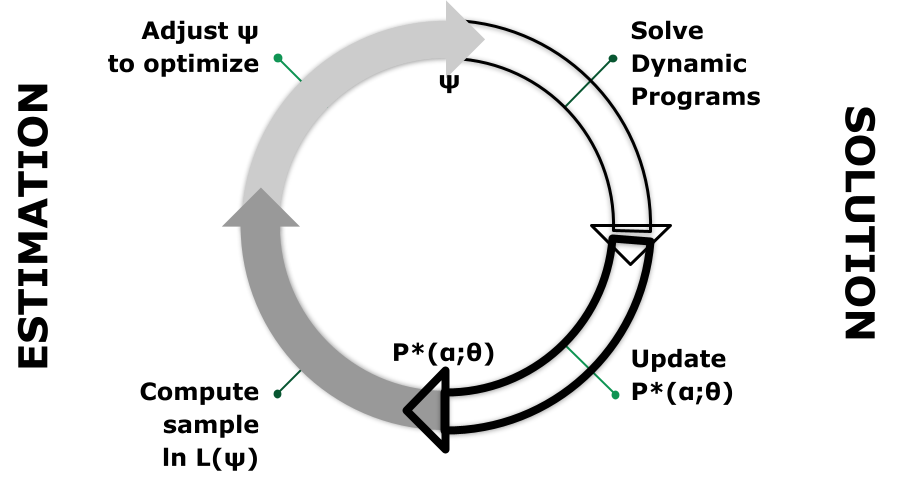
Most empirical DP uses variants of the nested algorithm introduced in Wolpin (1984) and illustrated as a two-sided feedback loop in 3. Given $\psi$ the DP model is solved and outcomes (CCPs) produced. Parameters are changed by a numerical optimization routine. It is this feedback that MaCurdy (1981) avoided by approximating the Lagrangian rather than computing its value based on the current value of the regression coefficients.
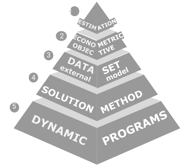
4 illustrates more layers of dependency. The top (or outer) level is an optimization algorithm that controls $\psi.$ The parameters are tied to an econometric objective at the next level down. Levels 1 and 2 correspond to the two sides of 3 which hides the layers below.
The objective relies on a data set (level 3) which must be organized to match the model to external data allowing for issues such as unobserved states and measurement error. Model outcomes and predictions use the DP solution method (level 4). Finally, the base of the pyramid is one or more DP models.
Each level of 4 must interface with the adjacent levels. The DP model must also access the structural vector $\psi$ controlled at the top level. niqlow provides classes for each level and the connective tissue between them. This integrated approach then supports automated construction of estimation problems. That is, the user need not write code for higher levels and can focus on the code at the base.
Estimation methods such as Aguirregabiria and Mira (2002)'s pseudo MLE and Imai et al (2009)'s MCMC estimation avoid computations within stages and swap the order of levels in 4. Dedicated purpose-built code to implement them looks very different than nested solution code. However, in niqlow the levels of 4 are modular. They can be re-ordered as long as different connections between objects representing each level have been written.
Previous sections used the labor supply model to demonstrate how to build up a DP as objects derived from the Bellman class, which corresponds to Level 5 of the pyramid. DP solution methods represent level 4. This section discusses how Levels 2 and 3 are represented in niqlow.
Outcomes and Predictions
Data related to a dynamic program are represented by theData class which has two built-in child classes. Data can be based on either outcomes or predictions. An outcome corresponds to the point when all randomness and conditional choices have been realized at a state. The complete outcome is a 6-tuple:
$$Y(\psi) \equiv \l(\matrix{ \phantom{y}&\al &\zeta &\eps &\eta&\th &\gamma_r &\gamma_f}\r).\label{Yagent}$$
Some elements of $Y$ are never observed in external data. In particular, the continuous shock vector $\zeta$ and the random effects vector $\gamma_r$ are treated as inherently unobserved. Only the agent knows these values at the point they choose $\al$.
Empirical work requires outcomes to be defined that mask components of the full outcome. Outcomes must also be put in a sequence to create the path of an individual agent. Unlike reduced-form econometrics empirical DP data cannot generically be represented as a matrix or even a multi-dimensional array of numbers. Instead, in niqlow they are stored as linked-lists of objects of the Outcome class. The next section builds on outcomes to define "generic" likelihood functions. The niqlow code is shown to estimate the simple labor supply model without the user coding the likelihood.
A prediction, on the other hand, is the expected value of outcomes conditional on some information. The basic prediction integrates over all contemporaneous randomness conditional on $\th$ and the permanent variables: $$E\l[Y\l(\th;\gamma_r,\gamma_f\r)\r] \equiv {\sum}_\eta {\sum}_\eps {\sum}_{\al\in A(\th)} f_\eta(\eta) f_\eps(\eps) P^{\star}(\al;\eps,\eta,\th,\gamma_r,\gamma_f) Y(\psi).\label{EYF}$$ This is what an agent expects to happen (in a vector sense) given that $\th$ has been realized but the IID state variables have not. The continuous shock $\zeta$ is integrated out by the choice probability $P^{\star}.$
As with outcomes, the information not available in the external data will not always match up with the conditional information in \eqref{EYF}. And predictions must be put in sequence to create a path. After discussing likelihod 5.5 returns to prediction and how they are used to construct GMM objectives.
Likelihood
There are three types of likelihood built intoniqlow depending on what aspects of the model are observed in the data. The types are labeled F, IID and PO. Each is a version of the full outcome $Y$ in which more information is masked or unobserved than in the previous version. The type of outcome must match up to the external data which is denoted $\hat{Y}.$
niqlow can determine which likelihood to apply automatically from the data read into an OutcomeDataSet object. The appropriate formula is computed without further user coding. Since each level of information relaxes the previous one, the PO algorithm could be applied to the other forms. Using the more restricted forms when possible speeds computation.
F: Full Likelihood
Define $Y^F$ as the full information outcome from the econometrician's point of view. It starts with $Y$ in \eqref{Yagent} then removes elements marked with $\cdot$: $$Y^F(\psi) \equiv \l(\matrix{ \phantom{y} &\al & \cdot &\eps &\eta&\th &\cdot &\gamma_f}\r).\label{YF}$$To build a likelihood function using full information, first assume there are no random effects variables so it is irrelevant that $\gamma_r$ is missing in $Y^F$. Then the likelihood for a single single observed outcome is the probability that the observed action would be taken: $$L^F\left(\ Y(\hat\psi)\ ;\ \hat{Y}\right) = P^{\,\star}(\hat\al; \hat\eps,\hat\eta,\hat\th,\cdot,\hat\gamma_f ).\label{LF}$$
This compact expression requires some explanation. The superscript has shifted to $L^F$ and the model outcome is shown with no superscript to avoid duplicate notation. On the right hand side is the conditional choice probability. This takes one of the forms in \eqref{CCP1}-\eqref{CCP3}.
Since the observed outcome includes the action and all state vectors, their data values are inserted into the conditioning values. niqlow integrates data and predictions so it inserts the observed values for the user. The model and external versions of the data illustrated in Level 3 of 4 correspond to $Y(\psi)$ and $\hat{Y},$ respectively. Calculations such as \eqref{LF} then enter an overall objective at Level 4.
All But IID Likelihood
Data rarely contain the full information outcome of a model as defined here. More common is the next case in which $\eps$ is unobserved. However, it is typical to observe additional function(s) of the full outcome to help identify parameters of the model. For example, in the labor supply model the earnings shock $e$ would probably be unobserved. However, earnings is observed if the agent worked. Extra information of this form is sometimes referred to as "payoff-relevant variables." Inniqlow they are referred to as auxiliary outcomes, and they are all placed in a vector $y.$
This leads to the third outcome type: $$Y^{IID}(\psi) \equiv \l(\matrix{y& \al & \cdot &\cdot &\eta&\th &\cdot &\gamma_f}\r).\label{YIID}$$ The auxiliary outcomes have been added to the front of the outcome. The agent has more information than $y$ so it is unnecessary for them to condition choices or transitions on $y.$ On the other hand, when the data is less than the agent's defined in \eqref{Yagent}, $y$ can contains additional information.
Both the smoothing shock $\zeta$ and the IID state $\eps$ affect the DP transition only through the choice of $\al.$ This means the IID outcome is sufficient to predict the next outcome as the agent would, namely using $P\st.$ Likelihood of a sequence of individual outcomes can be constructed that integrates only over the IID elements. The other IID vector in \eqref{ExtNotation}, $\eta,$ does not satisfy this condition because it can directly affect the transitions of other state variables.
The likelihood of an outcome when $\eps$ is unobserved is an expectation of $L^F:$ $$L^{IID}(\ Y(\hat\psi)\ ,\ \hat{Y}\ ) = {\sum}_{\eps} f\l( \eps\, |\, y=\hat{y} \r) L^F\l(Y,\hat{Y}\r). \label{LIID1}$$
The choice probability component is weighted by the conditional probability of $\eps$ given that it generates the observed value of $y.$ In this case \eqref{LIID1} can be discontinuous in $\psi.$ In the case of the labor supply model only observed earnings on one of the 15 points of support for $e$ would have positive likelihood. Further, if the set of discrete values of $\eps$ consistent with the model changes with a small change in $\psi$ it causes a jump in likelihood.
It is standard to add measurement error to observed auxiliary values (and other states or actions) in order to smooth out the IID likelihood. The measurement error is ex post to the agent's problem so it enters only at this stage: $$L\left(\ Y(\hat\psi) \ ;\ \hat{Y}\ \right)=P^{\,\star}(\hat{\al} ; \cdots )f(\eps)L_y(\hat{y},y). \label{LIID}$$
Here $L_y()$ is the likelihood contribution for the data given the model's predicted value for the auxiliary vector $y.$ As shown below, niqlow includes built-in classes to add normal linear or log-linear noise to any outcome's likelihood contribution derived from the Noisy class.
Path and Panel Likelihood
So far we have considered a single decision point in the DP model. In general, a path of outcomes for an agent is observed. The likelihood must account for stochastic transitions from one state to the next along the path. Denote a single outcome on the path as $Y_s$ and the path itself as $$\{Y\} = \left(\,Y_0,\,\dots\,,\,Y_{\hat T}\,\right).\label{Ypath}$$ The index $s$ is not necessarily the same as model time $t,$ and since $t$ is an element of $\th$ it does not need to be specified separately. The corresponding observed path is $\{\hat Y\}$ with ${\hat T}+1$ decisions observed. Random effects in $\gamma_r$ create permanent unobserved heterogeneity along a path which must be accounted for now.Let $g(\gamma_r)$ be the probability distribution of the random effects vector. The distribution can depend implicitly on $\gamma_f$ and $\psi.$ Multiple paths with the same fixed effects are stored in a "fixed panel." These fixed panels are concatenated across $\gamma_f$ in a "panel." A panel might hold simulated data only, but if external data will be read in then it is represented in niqlow by the OutcomeDataSet class.
Suppose the information available at a single decision is either full (F) or everything-but-IID as defined above. Let $\tau \in \{F,IID\}$ indicate which type of data are observed. Then the likelihood for a single agent's path is $$\eqalign{ L\l(\ \{Y\} \l(\hat\psi\r) \, , \,\{\hat{Y}\}\ \r) &= \cr {\sum}_{\gamma_r} g\l(\gamma_r \r){\prod}_{s=0}^{\hat{T}}& \l\{ L^{\tau}(Y_s,\hat{Y}_s)\times \left[ P\left(\hat{\th}_{s+1}; \hat{\al}_s,\hat{\eta}_s,\hat{\th}_s\right)\right]^{I\{s\lt \hat{T}\}}\r\}. \cr}\label{Lpath}$$
The rightmost term is the model probability for observed state-to-state transitions which only applies before the last observation on the path.
Efficient computation and storage of both the DP solution and this likelihood requires coordination. Placement of the "nested" solution algorithm must be exact. When there are fixed effects the model must be solved for the $G$ combinations of $\gamma_r$ and $\gamma_f.$ As discussed earlier, the endogenous state space $\Theta$ is not duplicated for each combination of permanent values. Otherwise storage requirements would multiply $G$-fold. On other hand, this means each combination must be fully processed for a given structural vector $\psi$ before proceeding to the next group. The fixed panel must initialize a vector to contain $L()$ for each of its members and then store partial calculations for $\gamma_r.$ Only when the outer summation in \eqref{Lpath} is complete can the log of the path likelihood be taken and summed across paths to form the log-likelihood. This must then be repeated for each fixed effects vector.
2-Stage Estimation
A version of ML estimation commonly known as two-stage estimation is available inniqlow (6). Since it was used in Rust (1987) two-stage estimation has been used to reduce the computational burden of maximum likelihood estimation. Parameters in the structural vector $\psi$ must be marked whether they only affect the transition of endogenous states or not. Consistent estimates of those parameters can be found without imposing Bellman's equation using the observed transitions.
More generally, in two-stage estimation each parameter is given one of the three markers by the user. The full parameter vector then contains three lists (sub-vectors): $$\psi = \left(\matrix{\psi_0& \psi_p & \psi_u }\right).\label{Subvecs}$$
The first, $\psi_0,$ contains parameters held fixed throughout estimation, including weakly identified parameters or ones set through "calibration." The second vector, $\psi_p,$ includes parameters that affect only transitions. The final vector, $\psi_u,$ contains parameters that affect utility and the discount factor $\delta$ if it is estimated.
At the first stage only $\psi_p$ is estimated using the limited information path likelihood: $$L^{1st} (\ Y(\hat\psi)\,,\,\hat{Y}\ ) = {\prod}_{s=0}^{\hat{T}} 1\times P(\hat{\th}_{s+1}; \hat{\al}_s,\hat{\th}_s)^{I\{s\lt \hat{T}\}}. \label{FirstStage}$$
This is the same as \eqref{Lpath} except "1" replaces the model's generated CCP. The likelihood conditions on the observed choice can be computed without solving Bellman's equation for $P^{\star}.$ The rest of the model setup is still required to compute the outcome-to-next-state transitions along the path. After estimating $\psi_p$ they are fixed at those values and $\psi_u$ is made variable. The likelihood reverts to \eqref{Lpath}. In niqlow a user implements 2-stage estimation with a few lines of code.
Type PO: Partial Observability
Implicit in \eqref{Lpath} are two assumptions. First, the initial conditions for the agent's problem are known up to $\gamma_r.$ Second, the full action and endogenous states in $\th$ are observed so that the likelihood only integrates and sums over IID values, $\zeta$ and $\eps.$ Calculation of $L$ can then proceed forward in time and the path, starting with $s=0.$More generally, partial observability of the outcome creates a difficulty for computing the path likelihood forward in time. Let $q$ be a state variable in the endogenous vector $\th$ that is unobserved in the data at outcome $Y_s.$ It could be missing systematically as a hidden state or incidentally for this outcome alone. It has a distribution conditional on past outcomes that can be computed moving forward. So the contribution to likelihood at $s$ can be computed by summing over possible values of $q$ weighted by its conditional distribution. However, the distribution at $s+1$ depends on the distribution of $q$ at $s.$ So the distribution must be carried forward in the calculation. Each unobserved value creates more discrete distributions to sum over.
Even if all the unobserved states are tracked and their joint distribution across missing information computed, this can still be inadequate to compute the correct likelihood. With $q$ missing at $Y_s,$ suppose also that the future point $s+k$ it equals $q^{\star\star}$ in the data. However, that value happens to have zero probability of occurring if $q=q^\star$ at $s.$ For example, if a stock was only at $q^\star$ at $s$ it may be impossible for the stock to grow to $q^{\star\star}$ by $s+k.$
Since $q$ was unobserved at $s$ the forward likelihood included $q^\star$ in the sum and the distribution. Now the contributions of paths that start at $q^\star$ must be eliminated between $s$ and $s+k.$ The likelihood must sum over only unobserved states conditional on past observed outcomes and future consistent outcomes. In general there is no way to calculate the likelihood forward when endogenous states or actions are unobserved.
Ferrall (2003) proposed 6 to handle partial observability. Instead of computing the likelihood of a path going forward in time, it is computed backwards starting at the last observed outcome ${\hat T}.$ At any point $s$ the likelihood computed so far is not a single number. Instead, likelihood is a number attached to every state at $s$ that is consistent with the observed data from $s$ forward. This avoids the trap of following paths forward that end up inconsistent with later outcomes.
A one-dimensional vector of likelihoods, denoted $L^{PO}_s,$ contains the information to track likelihood contributions farther in the future. If, at a particular $s$, the IID-level outcome is observed then this vector collapses to a single point. Encountering missing values for a smaller $s$ will expand the $L^{PO}_s$ to a vector again. The algorithm works for the special cases of Full or IID observability as well, but moving backwards is slower than algorithms that can move forward in $s$. When data are read into niqlow the user flags which variables are observed, and all other variables are treated as unobserved. As the data on the observed variables is read in incidental missing values are also detected. Then each observed path can be assigned one of the three tags $\tau \in \{F,IID,PO\}$ and the most efficient path likelihood is then computed.
- Construct $\Upsilon_0$ as outcomes consistent with the current observation on the path, $\hat{Y}_s:$ $$\Upsilon_0 \equiv \l\{ Y : Y \in \hat{Y}_s \r\}.\nonumber$$ Here "$\in$" means that the model outcome has the same values as the data.
- For all $Y \in \Upsilon_0$, define $$P(Y^\prime; Y) = \cases{ {\sum}_{\th\in Y}{\sum}_{\al \in Y} P^\star(\al;\th) L^{PO}_{s+1}(Y^\prime)& if $Y^\prime \in \Upsilon_1$\cr 0& otherwise.\cr}\nonumber$$ Transitions inconsistent with observations later in the realized path are zeroed out.
- Transition probabilities are multiplied by the conditional likelihood: $\forall Y \in \Upsilon_0$, $$L^{PO}_{s}(Y) \equiv L^{IID}\l( Y,{\hat Y}_{s}\r){\sum}_{Y^{\,\prime}} P\l( Y^{\,\prime}; Y\r).\nonumber$$
- Decrement s. Swap $\Upsilon_0$ and $\Upsilon_1.$
- If $s\ge 0$, return to step 1. Otherwise, handle initial conditions.
- If the clock is finite horizon (and simple aging), then $s=0$ corresponds to the first observed decision period, $t_{min}.$ If $t_{min}>0$ then the same process as above is continued but all outcomes are consistent with the data (because there is no data for $t\lt t_{min}$). If $t_{min}=0$ and $\Upsilon_1$ is a singleton, then its likelihood is the path likelihood. Otherwise, average the likelihoods of outcomes in $\Upsilon_1$ to collapse the path likelihood to a scalar.
- If the clock is ergodic, then optionally weight initial outcomes on path with the stationary distribution defined in \eqref{fstar}.
Estimating the Labor Supply Model
Consider using external data to estimate the parameter vector $\beta$ of the labor supply model. For simplicity other parameters are held fixed so we can set structural vector as $\psi = \beta.$ Data for individual $i$ is a path of the form: $$\l\{\hat{Y}\r\}^i = \l\{\ \l(m_s,M^o_s,E^o_s\r)\ \r\}_{s=0,\dots,\hat{T}^i}^i.\nonumber$$All work decisions are observed and there are no gaps in model time ($t_{s+1}=t_s$). Actual earnings, $E^a,$ depend on the observed work choice: $$E^a = \cases{ E() & if m=1\cr . & if m=0.\cr}\nonumber$$ The earnings shock $e$ is unobserved when not working. It could be inferred from $E^a$ except observed earnings, $E^o,$ include log-linear measurement error: $$E^o = e^{\nu}E^a,\quad \nu\sim N(0,\sigma^2).\nonumber$$
The auxiliary vector $y$ appearing in \eqref{YIID} contains $E^o.$ The observed path does not necessarily start at $t=0$. If it does, then observed experience $M^o$ equals actual experience because it can be computed from past work decisions before sending the data to niqlow. Otherwise, we'll assume that $M^o_0$ equals initial experience (acquired perhaps through retrospect questions). In this case \eqref{Lpath} is the likelihood for one observation with type $\tau=IID.$
To bring the simple labor supply model to this data, derive from LS a new class:
class LSemp : LS {
 static decl obsearn, dta, lnlk, mle, vi;
 static ActualEarn();
 static Build();
 static Estimate();
}LS is the parent class all its components are also in LSemp. LSemp does not declare Utility because its utility is the same as LS. The model is built using the code already included in the base LS class:
    LSemp::Build() {
1.      Initialize(1.0,new LSemp());
2.      LS::Build();
3.      obsearn = new Noisy(ActualEarn);
4.      AuxiliaryOutcomes(obsearn);
5.      CreateSpaces();
        }
The required Initialize() function is called on line 1. The only difference with the earlier call is that the state space $\Theta$ consists of LSemp objects not LS objects. The empirical version of the model shares the same set-up as the earlier version, so LS::Build() can be called on line 2. Observed earnings is created as an object on line 3. The Noisy class adds measurement error to the argument, actual earnings $E^a$ coded as a static function:
LSemp::ActualEarn() {
    return m->myEV() ? Earn() :.NaN;
}obsearn to the auxiliary outcomes, which makes it an element of the $y$ vector introduced in \eqref{YIID}.
The function for actual earnings requires some explanation. It uses Ox's .NaN code for missing values when not working ($m=0$). This is determined by m->myEV() instead of, say, $CV(m),$ which was explained earlier as returning the current value of m. That is used during Bellman iteration when $m$ is taking on hypothetical values.
At the estimation stage, however, the DP model must use the external value of actions to provide a predicted value of earnings. This was seen in the likelihood \eqref{LF} where the observed action $\hat\al$ enters the choice probability. niqlow handles this through its Data-derived classes that set values shared with the DP model. myEV() is another method of action and state variables. It retrieves the realized value of the variable if called during a post-solution operation such as likelihood calculation.
In ordinary econometrics, such as panel IV techniques, an endogenous variable is its own value. Only the value in the data is relevant. The need for CV() and myEV() reflects the complexity of nested estimation algorithms handled by niqlow and illustrated in 4. At the solution stage variables must take on hypothetical values to solve the model. At the estimation stage values from the external data set must be inserted into the contingent solution values such as the CCP.
Estimate() contains the code to compute the MLE estimates of $\beta,$ and selected output from it is discussed in Appendix D.
    LSemp::Estimate() {
1.      beta = new Coefficients("B",beta);

2.      vi = new ValueIteration();

3.      dta = new OutcomeDataSet("data",vi);
4.      dta -> ObservedWithLabel(m,M,obsearn);
5.      dta -> Read("LS.dta");

6.      lnlk = new DataObjective("lnlk",dta,beta);

7.      mle  = new BHHH(lnlk);
8.      mle -> Iterate();
}Parameter class designed to be manipulated by optimization algorithms. Like state variable objects, the value of the parameter is the v member of the class. Different classes constrain parameters in ranges of real numbers and vectors of related parameters like $\beta.$
In the basic model $\beta$ was an ordinary vector. Its value was set inside LS::Build() in D. In this version the goal is to estimate $\beta$ from data. So on line 1 its value is replaced. It now holds an object of the Coefficients class. This is designed to hold a vector of freely varying parameters like regression coefficients. A constant vector is needed as default for starting values. Since beta contains a vector before this line, its current value can be sent as the initial vector. By the end of line 1 that vector is stored internally in the object and beta now contains an object not a vector.
The code for the true earnings function LS::Earn() in E already included CV(beta). So when this model is estimated it will retrieve the values from the parameter object under the control of an optimization algorithm.
In the first use of the labor supply model the simple VISolve() function carried out Bellman iteration once. Its use of a solution method object was hidden from the user. Now that the solution method is nested within a likelihood calculation it is not enough. The vi member holds the value iteration object (line 2). Somehow this object must be embedded (nested) within the estimation procedure.
Lines 3-5 in K create the data set object. As illustrated in 4 this handles both external data and model predictions. The dataset object also needs to know which model outcomes are in the external data (implying other variables should be treated as unobserved). Line 4 says that $m$, $M$, and observed earnings are in the data and will have the same labels as their objects. Now the data can be read from a Stata file on line 5. A column in the external data must hold the ID of each path and the value of $t$ so that a panel of paths can be created. Since they were not set explicitly in the code, the default labels will be used and must appear in the data file to avoid an error. As Read() reads in the data it determines whether there are missing values along the path and what type of variable is missing (an element of $\eps$ versus other vectors that imply partial observability.) By line 6 the class of likelihood function for each path in the data has been determined.
The DP solution method created on line 2 of K has already been embedded at line 3, because vi was sent as the second argument when dta was created. Whenever a new likelihood evaluation is needed vi->Solve() will be called to re-solve the model. This is the "nesting" of the solution algorithm inside the sample likelihood.
Line 6 creates the econometric objective. DataObjective expects a data set such as dta to be sent to it. It has a built in method to compute the log likelihood. The objective is the "home" of the parameters to be estimated, $\beta.$
Lines 7 creates the algorithm to carry out the outer iteration of maximizing the likelihood. Note that the DP model is analogous to the econometric objective lnlk, and the Bellman solution method vi is analogous to the optimization algorithm. One difference is that the user's code must send lnlk to the optimization algorithm, whereas the value function method does not take an object.
This example uses the BHHH algorithm (line 7), which is Newton's method except the outer product of the likelihood's Jacobian matrix is used to approximate the Hessian. This happens without any special coding from the user because any Objective object has two methods for evaluating itself. One returns a scalar. The other returns a vector to be aggregated into the scalar. In this case, lnlk returns the vector of log-likelihoods for each observation. In turn BHHH uses the vector version to compute the matrix of partial derivatives with respect to $\psi$ and then the outer product.
Line 8 in K calls the Iterate() method of the BHHH object to maximize the log-likelihood starting at the initial values of $\beta.$ Values read in from a file can supplant the hard-coded starting values of beta. This is analogous to Method classes for different DP solution methods, each having a Solve() function to carry out the task on demand.
An additional 14 lines of executable code were used to estimate the simple labor supply model. The chains of interactions in the code segment above matches the stacking illustrated in 4. The DP model itself (the base level) is implicit, because only one state space can be defined. The user's code could substitute different classes at each level of the process without changing any other code. It can create different solution methods, load different data sets, or compare different optimization algorithms on the same objective. None of these changes require changing the underlying code for the DP problem as long as CV() and other preparations discussed above have been used to make the code ready for alterations.
Moments and Predictions
The example above uses MLE. The other main procedure used in empirical DP is GMM. In practice, GMM is used when the information a likelihood function requires is either missing or requires auxiliary assumptions the researcher wishes to avoid, such as imposing a conditional mean to be zero without assuming a full distribution of the error term.A prediction, denoted $E[Y],$ was defined in \eqref{EYF} as the integral over current IID randomness and conditional choices. Predictions always integrate over permanent random effects ($\gamma_r$) since they are treated as unobserved. Predictions always condition on permanent fixed effects ($\gamma_f)$ since they are treated as observed. Thus, for each $\gamma_f$, there is a single predicted path, although multiple outcome paths (used for MLE and data simulation) can be generated and/or observed in data for each $\gamma_f$. Concatenating prediction paths across different fixed effects produces a prediction panel.
Sequence of Predictions
To simplify notation, the description here will focus on only the endogenous state vector $\th$. Begin with an initial distribution over states, denoted $Q_0(\th).$ For example, if the initial state is given as $\th_0$ then this would simply be a vector of 0s and one 1: $Q_0(\th) = I\l\{\th =\th_0\r\}.$ Or, in a stationary environment the initial conditions might be the stationary distribution $Q_0(\th) = f_\infty(\th)$ defined in \eqref{fstar}.Now consider the distribution of $\th$ after $s$ decisions, $Q_s(\th).$ This distribution starts from $Q_0()$ and then accounts for the distribution of actions at 0 and the subsequent states at $1$ and so forth until $s$ actions have been taken. The prediction is the expected outcome over optimal conditional choice probabilities: $$E_s[Y] = {\sum}_{\th\in \Theta}{\sum}_{\al\in A(\th)} P^{\star}(\al;\th)Q_s(\th) EY(\al,\th).\label{EY}$$ Computationally this involves a loop over the state space and an inner product of the outcome and conditional choice probability vectors. Within the same loop, the distribution over states in the next period can be computed recursively.
$Q_{s+1}$ is accumulated over current state transitions: $$Q_{s+1}\l(\thp\r) = Q_{s+1}\l(\thp\r) + {\sum}_{\al\in A(\th)} P\st Q_s\l(\th\r).\label{Qs}$$ Once the prediction and next stage's distribution are computed, $s$ is incremented and the process repeated to form a path of predicted outcomes of a desired length.
Unlike path likelihood, which must deal with missing information along the path, $Y$ can be treated as the full outcome. A1 displays one element of $E_s[Y]$ vector, namely the action $m,$ along the path prediction for the simple labor supply. The full vector would also include the state $M.$ The exogenous states would by definition have time-invariant predictions and are not recorded in $E[Y].$ However, they can enter auxiliary outcomes which would be included in the prediction.
The external data may have missing information. Continue to define ${\hat Y}_s$ as the data but now is not an individual path but an average across ex-ante identical agents sharing a value of $\gamma_f.$ It includes only observed components of the outcome. To match empirical moments (averages) to the model prediction $E[Y]$, a masking matrix $M_s$ selects columns of the full outcome that are observed at stage $s.$ Then the differences between the predicted moment and the empirical moment is $$\Delta Y_s = \l( {\hat Y}_s - M_s{\hat E}_s\l[Y\r]\r).\label{DeltaYs}$$
Masking is applied to the predicted moment only to make it conform to the external data vector.
GMM Objectives
Returning to the differences between averaged data (moments) and predictions defined in \eqref{DeltaYs}, concatenate them along an observed path: $$\Delta \{Y\} = \left(\matrix{ \Delta Y_0 \cr \Delta Y_1 \cr \vdots \cr \Delta Y_{\hat T}}\right).\label{DeltaY}$$To form an econometric objective the vector of differences is aggregated into a scalar value. There are 3 types of GMM objectives built into niqlow. The simplest case is a weighted sum of all differences:
$$J_0 = -{\sum}_{s=0}^{\hat T} \l\| {\sum}_{j=1}^J \omega_{sj} \Delta Y_s^j \r\|.\label{J0}$$
The negative sign appears because objectives are maximized. The user specifies the weights $\omega_{sj}$ to place on each observed moment $j$ at each point $s,$ including an option to set all weights equal. These weights can also be ad hoc "importance" weights. Further, the number of observations averaged at each $s$ can be read in so that weights also account for precision in the empirical moments. If the model includes different observed groups ($\gamma_f$) there is a summation over their separate values of in \eqref{J0} and the subsequent forms.
The next option is to specify a matrix or matrices to account for contemporaneous correlations between observed moments: $$J_1 = -{\sum}_{s=0}^{\hat T} \| \Delta Y_s\ \Omega_s\ \Delta Y_s\|.\label{J1}$$
Finally, efficient GMM requires that a weighting matrix for the full path of moment differences: $$J_2 = \Delta\{Y\}\ \Omega\ \Delta\{Y\}.\label{J2}$$
The efficient matrix $\Omega$ can be computed from individual data if available and the empirical moments are computed from them. However, this is not helpful if GMM is used because only moments over individual paths are available. niqlow includes procedures that will simulate individual paths and then compute $\Omega$ from them using a first-stage (consistent but inefficient) parameter vector.
The previous section discussed all the code involved in estimating the labor supply model using MLE. Much of that code would remain if GMM were used instead. The key differences would be a single statement:
momdta = new PredictionDataSet(UseLabel,"avgdata",vi);vi is the nested solution method object to be called whenever the objective will be re-computed. This also specifies the default weighting scheme in \eqref{J0}. The statements to match outcomes to data columns, create the data objective and read in the data are essentially the same as with MLE.
Roadblocks
Return to the question posed earlier: Why does MaCurdy (1981) now take one Stata command but Wolpin (1984) still requires purpose-built code? First, MaCurdy (1981) keeps data, model predictions, and estimated parameters from having multifaceted roles. Dynamics is concentrated into the Lagrange multiplier which can be approximated as a fixed effect. Hours of work, while a choice within the lifecycle model, only enters the model as an observed data point. Tracking other contingent choices are not required. Thus, hard-wired code for panel IV and other similar methods could move towards an OOP approach as followed by Stata, R and other current platforms.In Wolpin (1984) the binary choice prevents dynamics from concentrating into a Lagrange multiplier. Estimated parameters are not just coefficients on observables. Instead they enter choice probabilities through their effect on the value function. Choice probabilities are contingent, and the observed choices determine which ones enter the likelihood. When faced with these data and parameter interactions no software emerged to assemble a DP model and derived its empirical content from pre-defined components.
Empirical DP remains compute bound: processor speed is a limiting factor to the scale of the model. Custom-built compiled code can be the most efficient in execution speed. But the interlocking roles of data and parameters illustrated in 4 results in "hard-wired" details for the given model. A change in the model requires rewriting deep code.
Reduced-form estimation is not as computationally intensive and lacks hidden layers such as solving Bellman's equation to compute choice probabilities. This research could move to platforms such as Stata even when it was restricted in storage and speed compared to purpose-built compiled code. Meanwhile, empirical DP continued to require fast single-purpose code for each application. Once complete there is little incentive to return to the code and make it general, which would be difficult for the reasons given above. Even when code is freely shared with others it is of limited use to someone building a different but related model. So, unlike panel IV estimation represented by MaCurdy (1981), no natural shift occurred from bespoke PP code to use of off-the-shelf OOP components for the empirical DP approach introduced by Wolpin (1984).
To overcome this roadblock, niqlow did not start from purpose-built code. Instead, it started with OOP representations of generic DP models before solving a single specific model. Classes encode features of elements independent of the rest of the model so the model can be built from components. This creates computational overhead compared to, say, nested loops in a compiled language. However, as discussed in 3.3, efficiencies in the design of niqlow are coded once-and-for-all. Integrated data and optimization tools further reduce specialized coding.
Custom-built, expertly-tuned code for a single problem will always run quicker than equivalent code in niqlow if the starting line for the comparison is set to when programs start executing. If, instead, the starting line is set at the first attempt to build the model then time-to-completion is likely to even out.
Conclusion
This paper introduces an approach to empirical dynamic programming that eliminates the need for custom coding of each project.niqlow is an open-source platform that uses object oriented programming (OOP) to provide its user a set of tools to design, solve and estimate a model. It recognizes that empirical DP involves multiple phases: computing the value function; updating choice probabilities; evaluating the likelihood for data; adjusting parameters to find consistent estimates; and finally simulating the effects of policy experiments. To accomplish these phases the niqlow user need not re-invent the wheel. Instead their code consists primarily of high-level statements that select off-the-shelf components of standard models.
There is little evidence from the literature that sharing purpose-built code for a published paper has promoted verification or direct extension of already published empirical DP work. Referees of empirical DP models are also rarely in a position to replicate results reported in manuscripts. Finding bugs in purpose-built code for a large empirical DP model is never going to be practical. At best, referees can point to discrepancies in output that might be caused by mistakes that the authors can work to resolve.
Results generated from empirical DP papers have played at best an indirect role in shaping policy. One reason for this is skepticism among researchers not performing empirical DP themselves. Results are opaque, not independently verified, and rarely subject to robustness checks. Thus, a conundrum exists: empirical DP results are not trusted in part because they are based on purpose-built code that is rarely if ever verified. Because the results are not trusted they rarely play a role in policy debates. Since they do not influence policy, unverified results stay unverified for lack of relevance.
Perhaps niqlow is a step towards closing the structural coding gap, which lowers the cost of producing new results and replicating old ones. This in turn may make results more relevant and comparable to reduced-form methods already produced by portable and easy to use code.
Notes
https://quantecon.org/) is a collective effort to create useful tools.niqlow is written in Ox, which is free for research purposes and runs on most systems. Current niqlow syntax is used here and the code is included in the examples in niqlow distribution. The current version has no graphical user interface or menu system, but the OOP approach makes it straightforward to build one.niqlow is placed on discrete actions and discrete states, but some elements of the core code includes continuous state variables and continuous choices can be incorporated. Methods for continuous time models can be added as well.niqlow.niqlow also includes model classes based on normally distributed additive shocks, both ex ante and ex post. Transit() method which returns a pair of values: a vector of feasible integer values next period and a matrix of transition probabilities corresponding to feasible actions (rows) and feasible state values next period (columns). Because $M$ was added to the model its Transit() function will be called at each state along with all other transitions. The transitions for all state variables are combined to form $P(\thp;\alpha,\th)$ which ends up as a vector of feasible state indices and a matrix of probabilities.In an ordinary lifecycle model $T-1$ is a final period, but under this clock the agent stays in the final period forever. Also, a lifecycle model might incorporate early mortality:
$$t' = \cases{ t+1 &prob. $1-\lambda(\th)$\cr
T-1 &prob. $\lambda(\th)$\cr}\label{mort}$$
The last period $T-1$ is death which may have an intrinsic value (such as bequests). The current value function depends on values for two different future times, $t+1$ and $T-1.$ These and other clocks are built into niqlow.
niqlow stores the transition $P\l(\thp;\al,\th\r)$ at each state because they are needed for simulation and prediction. The transitions are stored for each $\th$ using a sparse method that tracks only feasible new state indices and the vector of probabilities conditional on choices. The transitions of the IID vectors $\eps$ and $\eta$ are stored once and combined with the $\th$ transition to determine the full state-to-state process.niqlow uses Ox-specific syntax to reduce select only relevant matrix elements to process. Using an interpreted language such as Ox includes overhead, but features of the syntax such of this can result in fast as well as simple and general code.VISolve() function can only be used with heterogeneity to solve the problems. Use of the solved solutions requires nesting the a solution method within the use of the solution as discussed 5.4.niqlow allows the user to control these and other details of the model.niqlow avoids this altogether by mapping a multidimensional space into one dimension. That is, if $\th$ is a vector of state variable indices, then the state's one-dimensional index is $I\th$, where $I$ is a row vector of offsets that depend on the number of values each state variable takes on. In addition, as in other interpreted languages, the length of a vector such as $\theta$ can be set dynamically during runtime in Ox.Appendix
Appendix A. Example of PP vs. OOP Coding
To illustrate differences between OOP and PP, consider a package written by a programmer to be used by economists (users): first using the PP paradigm only and then using OOP. The package, namedMarshall, solves for Marshallian demand for a consumer with utility $U(x)$ defined on a vector $x$ and a given price vector $p$ and income $m:$
$$x^\star(p,m;U)\quad\equiv\quad {\arg\max}_{\ x: px\le m\quad} U(x).\nonumber$$
Most readers have probably coded an objective and then called a built-in optimization procedure to optimize that function. Marshall is a specialized version of that general problem.
The PP package documentation explains how users should code $U()$ in order to interact with tools in the package. The user codes u(x), and sends it to a built-in procedure of the form demand(u,p,m). That procedure uses algorithms to compute $x^\star(p,m).$ Suppose the user wants to use the Cobb-Douglas function, $U(x) = {\sum} \ln x_i.$ Using "pseudo-code" the key parts of the user's program might look like:
#uses Marshall
u(x) {
    return sum_i ln(x[i])
    }
qdemand = demand(u,prices,income)
print("x* = ",qdemand)
class Consumer {
    members
                xstar, p, m
    methods
                demand()
                budget(p,m)
        virtual u(x)
}u(x) belongs to the Consumer class and does the work of computing utility. The budget parameters are stored as members of the class. These will be set by passing them to the budget() method. The method demand() is the same as the PP procedure above, but it will get the information it needs from the data members rather than from arguments. It stores the result in the member xstar.
The package comes with the Cobb-Douglas function set as the a default to demonstrate the package without any coding. Now $u()$ is coded as a method of the Consumer class:
Consumer::u(x) {
    return sum( log(x) )
}u() has the prefix of the class it belongs to. Code for the other methods would also be part of the package. User code to create a Consumer object, set the budget to already-defined values, and solve for $x^\star$ might look like this:
#uses Marshall
    ⁞
agent = new Consumer()
agent -> budget(prices,income)
agent -> demand()
new operator makes an object from the Consumer template and stores it in the variable agent. The code above would use the built-in utility and compute quantity demanded at the prices and income sent to the budget operator. The syntax object -> method() is a common way to invoke a method for a particular object. That is, instead of sending $u$ to demand() in the PP approach, the data specific to agent is automatically available to the demand() method belonging to agent.
The code so far uses a built-in utility. To use, say, a CES utility the user creates a class derived from Consumer.
class CES : Consumer {
    members  a
    methods  u(x) CES(ina)
    }
CES::CES(ina) {     a = ina    }
CES::u(x)     {     return sum_i (x[i]^a)^(1/a)    }
⁞
agent = new CES(0.2)
agent -> demand()
⁞CES is a child of Consumer. The new class does not declare its own demand() method, because CES inherits the version from Consumer. The user also provides a method that is called to create a new object. This constructor has the same name as the class in the pseudo code. The CES parameter is passed to it and stored in CES.a, ready to be used by CES::u().
When demand() is invoked, the user-provided CES::u() is called instead of the default version written by the programmer. The user has not changed, and perhaps cannot even see, the original code for demand(). This is because the programmer marked Consumer::u() as virtual. By doing so the programmer gives the user a controlled ability to change the underlying code through insertion a replacement function. In the PP packaged this injection of code was accomplished by passing u to the demand function. When many functions need to be replaced in many algorithms the PP framework can become unwieldily and unreliable. The OOP approach scales more efficiently for both the programmer and the user with problem complexity. With OOP it is easier to ensure the right data and the right functions are being used within the package.
The programmer can create a taxonomy of classes for the user to choose from. In this simple case, Marshall might not just have a single Consumer class. It might have child classes for different classes of utility. The user can then start with one of those classes to specialize or extend it for their model. An OOP package can provide the user with a menu of options, an important part of the niqlow approach to empirical DP.
Appendix B: Code Segments and Additional Explanation of niqlow Features.
$CV()$ and $AV()$ in Code Segment E
If the action counter $M$ were an ordinary programming counter taking on values between 0 and 39 then the statement E.1 would not require sending it to CV(). A simple assignment D=M would set D to the current value of M. However, M is an object of a class so it is not the same as its value. Instead, the current or counter value of $M$ is a member of the object. Classes in niqlow that represent DP variables have a member v that holds the counter or current value of the variable. The internal code sets the value of v to correspond to the current state $\theta$ before code such as Utility() is called. The function CV(M) returns M.v. So either D=M.v; or D=CV(M); is how user code would set D to the value of $M$ at the current state.
Recall that utility is treated as a vector valued function corresponding to the feasible set $A(\th).$ Since $m$ is an action variable its current value is not a scalar at $\theta.$ In this simple one-choice model the current value is always the same: $CV(m) = \l(\matrix{0\cr 1}\r).$ If other actions were added, or if constraints on feasible actions were imposed on choice, the current value of $m$ would be a different length because the number of distinct actions $\alpha$ would change.
Since $M$ is a simple count variable, it takes on values like a loop counter or index. The earnings shock $e$, is also like a loop counter, so its Its counter value ranges from 0 to 14. However, $e$ is a discretized normal random variable and the counting values are associated with both positive and negative real numbers, i.e. quantiles of the standard normal distribution, such as $-1.282,$ the 10th percentile of $N(0,1)$. The user's code can carry out these transformations of the integer value e.v, but niqlow can track actual values of variables for the user.
The actual values of an object are stored as vector member actual. Thus the actual value at any point is actual[v]. The current value is an index into the actual vector. The function AV() function retrieves this value, so when $CV(e)=3$ $AV(e)$ might equal -1.282. For $M$ the actual vector is (0 1 … 39) and actual[v]=v. That is, the default is that AV(s)=CV(s). Only in the case like a discretized normal will there be a difference. The user can set actual values for their state and action values and can make them dependent on structural parameters.
Semi-Exogenous State Variables
An example of an IID process that could be sorted into $\eta$ but not $\eps$ is a wage offer $h$ with on-the-job search. If the offer is accepted it determines earnings this period also the existing wage next period. The existing wage is then a state variable placed in $\th$ because its transition depends on choices. Next period a new IID outside shock $h$ is realized as well, but current $h$ affected the transition beyond its influence on the action $\alpha$ so it must be placed in $\eta$ not $\eps.$
acc = new BinaryChoice("acc");
offer = new  LogNormal("offer" , 10);
curw = RetainMatch(offer,acc,1,0);
ActionVariable(acc);
SemiExogenousStates(offer);
EndogenousStates(curw);
Additional Actions and Restricted Choices
Starting with the basic labor supply model suppose the user wants to add a choice to attend school or not ($s$) and a state variable to track accumulated schooling: $S^\prime = S + s.$ The agent cannot attend school and work in the same period, so the choice vector and feasible set are now $$\alpha = \l(\matrix{s & a}\r) \in A(\th) \equiv \l\{ \alpha:\ s*a = 0\r\}.\nonumber$$ Although initialization and space creation can only occur once, in between new variables can be added to the vectors more than once. So the extended build is simply:
LSext::Build() {
    ⁞
    LS::Build();
    s = new BinaryChoice("att");
    S = new ActionCounter("sch",8,s);
    Actions(s);
    EndogenousStates(E);
    ⁞
}m to the action vector. This adds s to it. S is an action counter like M but limited to 8 years of additional schooling to reduce the size of the state space.
The user must tell niqlow to impose the condition that the agent can either work or study but not both. This creates an additional trimming of unreachable states: $M+S\le t.$ In this approach the agent has to impose this extra condition on reachable states. The user replaces two built-in virtual methods with their versions:
LSext::FeasibleActions() {
    return CV(m) .* CV(s) .== 0;
    }
LSext::Reachable(){
    return CV(M) + CV(S) <= I::t;
}niqlow places its current value in the I class, so I::t is always available as well as other indices of the current state.
Augmented State Variables
The current library of pre-defined state variable types inniqlow include counters, accumulators, lagged values, durations, and discrete jump processes. A user can also provide a Markov transition matrix for an arbitrary process. Many estimated DP models contain state variables that customize these basic versions. For example, some models may "freeze" a state variable at it's current value after some period $t^\star.$ In some models a state variable stops being relevant to the agent's problem at some point. For example, a model of schooling and work might track credits earned while still in school, but once out in the labor market credits no longer matter and tracking them is inefficient. These are called augmented state variables in niqlow.
Here are 3 augmented state variables:
    x = new Freeze( new ActionCounter("sch",8,s), 15 );
    y = new Reset(b,a);
    z = new ForgetAtT( new ValueTriggered(d,tvar,1,5), 20 );
Freeze which then wraps the augmented transition rules around the base transition.
State variable $y$ augments a base state variable $b$ (not shown here) so that its value resets to 0 whenever the agent sets the action variable $a$ to 1 (also defined elsewhere). This is a special case of the general Triggered() augmentation. Several triggers besides the simple reset are already coded. Finally, z is a double augmentation of a state variable $d$ and another state variable $tvar.$ . First, when tvar=1 $z$ will reset to 5. From $t=20$ and onward the value of $z$ is not tracked because of the ForgetAtT augmentation. Forgetting a sate variable means its value is simply $CV(z)=0$ from then on, which avoids expanding the state space unnecessarily.
Complete Code and Output for the Labor Supply Example
This Ox code is available in theexamples folder in the niqlow download. A few lines are different than the code in the main body to account for the reservation wage extensions.
#import "niqlow"
class LS : ExtremeValue {
    static decl m, M, e, beta, pi;
                Utility();
    static      Build(d=FALSE);
    static      Create();
    static      Earn();
    }
main() {
    LS::Create();
    VISolve();
    ComputePredictions();
    }
LS::Build(d) {
     SetClock(NormalAging,40);
     if (isint(d)) {
        e = new Nvariable ("e",15);
        m = new BinaryChoice("m");
        Actions(m);
        ExogenousStates(e);
        }
     else
        m = d;
     M = new ActionCounter("M",40,m);
     EndogenousStates(M);
     SetDelta(0.95);
     beta =<1.2 ; 0.09 ; -0.1 ; 0.2>;
     pi = 2;
    }
LS::Create() {
    Initialize(1.0,new LS());
    Build();
    CreateSpaces();
    }
LS::Earn() {
    return  exp( (1~CV(M)~sqr(CV(M))~AV(e)) * CV(beta) ) ;
    }
LS::Utility() {
    return CV(m)*(Earn()-pi) + pi;
    }
 t           m           M                 t           m           M
  0      0.3982      0.0000                20      0.1540      4.9016
  1      0.3761      0.3982                21      0.1508      5.0556
  2      0.3537      0.7743                22      0.1480      5.2064
  3      0.3319      1.1279                23      0.1456      5.3545
  4      0.3111      1.4598                24      0.1434      5.5000
  5      0.2918      1.7709                25      0.1414      5.6434
  6      0.2741      2.0628                26      0.1397      5.7848
  7      0.2580      2.3369                27      0.1382      5.9246
  8      0.2434      2.5949                28      0.1369      6.0628
  9      0.2303      2.8383                29      0.1358      6.1997
 10      0.2186      3.0686                30      0.1348      6.3355
 11      0.2082      3.2872                31      0.1339      6.4703
 12      0.1989      3.4954                32      0.1332      6.6042
 13      0.1907      3.6944                33      0.1325      6.7373
 14      0.1834      3.8850                34      0.1320      6.8699
 15      0.1769      4.0684                35      0.1316      7.0019
 16      0.1712      4.2453                36      0.1313      7.1335
 17      0.1661      4.4165                37      0.1310      7.2648
 18      0.1615      4.5825                38      0.1309      7.3958
 19      0.1575      4.7441                39      0.1308      7.5267
In this model we can push the smoothing parameter from 1.0 to near 0 and to very large:
    Initialize(1.0,new LS());         Baseline
    Initialize(0.001,new LS());       Near perfect smoothing
    Initialize(100.0,new LS());       Almost no smoothing
    SetDelta (0.95);                  Baseline
    SetDelta (0.0);                   Static decisions
    beta = <1.2 ; 0.09 ; -0.1 ; 0.2>;   Baseline
    beta = <1.2 ; 0.0; 0.0; 0.2>;       Static environment (no experience)
Once the extremes are confirmed we can deform the problems slightly and see that the output moves in the right direction.
Unlike purpose-built code, in niqlow these kinds of tests use the same underlining code for all models. In addition, the behavior of a state variable class, such as ActionCounter can be confirmed in a small test program. Then it is very likely it will perform correctly in any other problem.
Certainly not all bugs have been discovered let alone fixed in the current niqlow code. And varying parameters of a single model will not reveal all errors. However, as changes are made that might break code that used to work, a suite of test programs are run to make sure that output is still correct. In that sense the changes to experiments on the labor supply model are important for a user to run in order to overcome healthy skepticism. However, the kinds of errors that might uncover have been squashed by checking test program output that include many other features than the labor supply model but in smaller spaces. There are also debugging features that can be turned on to trace output when a bug has been discovered.
Appendix C: Solution Algorithms
These algorithms are explained in 4.2. Aguirregabiria and Mira (2011) review several methods in more detail.SetP is initially FALSE. A new flag, SetPtrans also starts as FALSE.SetP=TRUE and SetPtrans=TRUE to compute the state-to-state transition \eqref{Pqtoq} on each iteration.- Compute $$\eqalign{ \overrightarrow{\Delta}_t &\equiv Emax(V_1) - V_1\cr g &\equiv \left(I-\delta P(\thp;\th)\right)^{-1}\left[\overrightarrow{\Delta}_t\right]\cr V_0 &= V_1 - g\cr}\nonumber$$
- For all $\theta \in \Theta_t$:
- Store action values at a single $\eps_0$ (the median or mean vector): $v_0(\al,\th) = v(\al;\eps_0,\th)$ and
maxE$= V_0(\th)=\max v_0(\al,\th).$- if $\th \in \Theta_t^S$, compute
Emax$= V$ , averaging over all values of the IID state vector $\eps$: $$V(\th) = {\sum}_{\eps} \ \l[ {\max}_{\ \al\in A(\th)\ }\ U\l(\al;\eps,\th\r) + \delta E_{\,\al,\th\,}V\l(\thp\r)\r]\ f\l(\eps\r).\nonumber$$ - Store action values at a single $\eps_0$ (the median or mean vector): $v_0(\al,\th) = v(\al;\eps_0,\th)$ and
- Approximate $V$ on $\Theta_t^S$ as a function of values computed at $\eps_0$. The default runs the regression:
$$\hat{V}-V_0 = X\beta_t =\l(\matrix{\l(V_0-v_0\r) & \sqrt{V_0-v_0}}\r)\beta_t.\nonumber$$
That is, the difference
Emax-maxEis a non-linear function of the differences in action values at the median shock. - For $\th \not\in \Theta^S_t,$ compute $v_0(\th),$ extrapolate the approximation: $$V(\th) = \max\{ V_0(\th), V_0(\th)+X\hat\beta_t\}.\nonumber$$
KeaneWolpin class.Appendix C: Reservation Values
For a binary choice $a$, there is a single $z^\star$ at each (implicit) state that solves $v(1,z^\star)-v(0,z^\star) =0.$ Let $EV_i$ denote $EV\l(\thp\,|\,a=i\r)$. After some rearranging $z^\star$ satisfies $$U(1,z^\star)-U(0,z^\star) = \delta\l[ EV_0-EV_1\r].\label{WS1}$$ The differences between current and future values balance, and \eqref{WS1} are solved as a non-linear equation. The condition that future expected values cannot depend on current $z,$ avoids a more complicated condition. Each additional choice beyond binary adds another equation between adjacent values to be solved simultaneously.Once $z^\star$ has been found, Bellman iteration requires calculation of the expected value of arriving at the (now explicit) state $\th:$ $$\eqalign{ EV(\th) = G(z^\star)&\l( E\l[U|a=0,z\lt z^\star\r] + \delta EV_0 \r)\cr + \l(1-G(z^\star)\r)&\l( E\l[U|a=1,z\ge z^\star\r] + \delta EV_1 \r).\cr\label{EVz} }$$ These conditions are illustrated in A2. Conditions \eqref{WS1}-\eqref{EVz} include three additional objects that the user's code must provide. The first condition for $z^\star$ needs $U\l(A(\theta),z\r),$ a vector of utilities for candidate values of $z$ while solving for $z^\star.$ The second includes $F(z^\star)$ and the vector of expected conditional utilities, $E\l[U\l(0\r)| z\lt z^\star\r]$ and $E\l[U\l(1\r)|z\ge z^\star\r].$
The model must satisfy several conditions described there to be eligible for this solution algorithms. These are enforced by allowing only models derived from the OneDimensionalChoice class to use the ReservationValues method.
- $\al$ must be one-dimensional (only one variable added to the action vector);
- No smoothing shock $\zeta$ is included (because $Z$ plays that role);
- No state variables are placed in $\eps$ and $\eta$ vectors (because reservation values must be stored using $\th$);
- Choice values $\vv$ must the single-crossing property.
OneDimentionsalChoice adds two virtual functions that other Bellman classes do not. The two functions are Uz() and EUtility(). At $z^\star$ the difference in current utility equals the discounted difference in future values. The user codes Uz(z) to return utility of all choices at $z$. The reservation value solution method uses that to solve for $z^\star.$ Backward induction requires the expected utility of each option conditional given the optimal value $z^\star$, hence the need to provide EUtility().
Continuous() method. If so, create storage for $z^\star$ at $\th.$- At each $\th \in \Theta_Z$ initialize $z$ solve for $z^\star$ based on the user-provided $Uz(A(\th);z).$ When completed store $z^\star$ at $\th.$ Use
EUtility()that provides $F(z^\star)$ and $E[U|A(\th),z^\star]$ to compute $V(\th)$ based on \eqref{EVz}. - For $\th$ not in $\Theta_Z$ compute $V(\th) = U(\al;\th) + \delta EV(\thp)$ as in Bellman iteration but with a single action available.
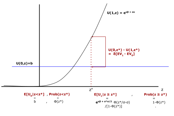
Code for the Reservation Value Labor Supply Model
For the basic labor supply model, the earnings shock $e$ is a discretized normal. Change that assumption so it is a continuous standard normal random variable, re-labeled $z.$ The class created for this version will be namedLSz. Earnings are now written
$$E = \exp\{\beta_0+\beta_1M +\beta_2M^2 + \beta_3 z\}.\nonumber$$
Since $E$ exceeds the value of not working ($\pi$) for large enough values of $z$ there is a reservation value for the choice $m=1.$ Since LSz must be a one-dimensional choice model it cannot be derived from LS as was done earlier with LSext.
However, code from the basic model can be reused because most elements of LS are static. The only non-static member was Utility(). By using the static elements a change to LS will still be reflected automatically in LSz. In particular, LSz::Uz() can use LS::Earn() to utility at $z$. First set the value of LS::e to z then calls LS::Earn().
In the model expected utility of not working is simply $\pi$. For working, expected utility involves $E[e^{\beta_3z}|z>z^\star]$. The Mills-ratio formula for log-normality gives expected utility conditional of acceptance as $$E[U|m=1,z>z^\star] = \exp\l\{\beta_0+\beta_1M+\beta_2M^2+{\beta_3^2\over 2}\r\}{\Phi\l(z^\star/\beta_3 - \beta_3\r)\over \Phi\l(z^\star\r)}.\label{EU}$$
The constant factor includes $\beta_3^2/2$, because it is coefficient on the normal random variable $z$ (and hence the variance of the model shock). The ratio of $\Phi()$ values is new to the continuous specification and can't be borrowed from the discretized LS.
However, note that only the constant term includes the Mincer equation, and it is the same as the original earnings function if $e=\beta_3/2.$ So again the base LS::Earn() function can be used by setting the value of e first. Thus, even though LS was coded for a completely different approach its specification is still synchronized with the reservation wage version. Only elements specific to the new version need to be coded.
This code segment converts the labor supply model to a continuous choice reservation value problem.
#include "LS.ox"

class LSz : OneDimensionalChoice {
    static Run();
    EUtility();
    Uz(z);
    }
LSz::Run() {
    Initialize(new LSz());
    LS::Build(d);
    CreateSpaces();
    RVSolve();
    ComputePredictions();
    }
LSz::Uz(z) {
    LS::e = z;
    return LS::pi | LS::Earn();
    }
LSz::EUtility()    {
    decl pstar = 1-probn(zstar),
         sig   = LS::beta[3];
    LS::e = sig/2;
	return {  ( LS::pi | LS::Earn()*probn((zstar/sig-sig)/pstar))
              , (1-pstar)~pstar
            };
	}
Appendix D: Estimation on Simulated Labor Supply Data
Code segment K estimated the labor supply model from external data. To use simulated data the code is modified slightly:
    dta = new OutcomeDataSet("data",vi);
    dta -> Simulate(1000,40);
    dta -> ObservedWithLabel(m,M,obsearn);
Abbreviated output is below. The code detects that none of the observations are full CCP because $e$ is unobserved. Since all actions and endogenous states $\th$ are observed all paths are categorized as IID. This means niqlow will automatically sum over $\eps$ to compute the likelihood but it is unnecessary to use the backward Algorithm 6. The measurement error on noisy earnings is fixed at its true value. The result is convergence after 5 BHHH iterations with weak convergence. Because by default niqlow scales starting parameters the reported standard errors would need to be re-scaled, or recomputed with scaling and constraining turned off (details available in the documentation). Having started at the true parameter values, the sample likelihood is within .01% of the initial value with some differences in parameter estimates, particularly the coefficient on experience ($M$).
Masking data for observability.
Path like type counts
    CCP    IIDPartObs
      0   1000      0
Report of Gradient Starting on lnklk
   Obj=          -29378.9180146
Free Parameters
         index          free
B0         0     1.00000000000
B1         1     1.00000000000
B2         2     1.00000000000
B3         3     1.00000000000
Actual Parameters
                  Value
B0         1.20000000000
B1       0.0900000000000
B2       -0.100000000000
B3        0.200000000000

1. f=-29375.8 deltaX: 0.32545 deltaG: 50.0006
        Output for iterations 1-4 removed
5. f=-29375.8 deltaX: 4.45343e-05 deltaG: 0.00906749

Finished: 3:WEAK
                          B0           B1           B2           B3
    Free Vector       1.0485      0.66901      0.97388      0.93059
    Gradient     -3.3945e-05  -4.1913e-05   0.00017144   1.0543e-05
   Std.Error        0.022743      0.14097     0.014054      0.18729

Report of  Iteration Done  on lnklk

   Obj=          -29375.7501799
Free Parameters
         index          free                  stderr
B0         0     1.04850905614   0.0227425353445
B1         1    0.669005636205    0.140973390182
B2         2    0.973884754314   0.0140539379652
B3         3    0.930592373935    0.187285663731
Actual Parameters
                  Value
B0         1.25821086737
B1       0.0602105072584
B2      -0.0973884754314
B3        0.186118474787