- A Two Person, Two Good Exchange Economy The Edgeworth Box is a century-old way to visualize the fundamental interaction in economic theory: gains from trade of scarce resources.
- Pareto Allocations and the Core The slope of the indifference curve is called the marginal rate of substitution (MRS). I hope that readers remember that the MRS equals the ratio of the marginal utilities: $$MRS^i(x^i) = -{\partial U^i(x^i) / \partial x^i_0 \over U^i(x^i) / \partial x^i_1}.\nonumber$$
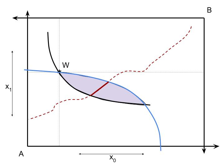
- Competitive Allocations The contract curve can be thought of as the prediction of what would happen if A and B negotiate face to face. Neither would voluntarily trade to a point with a utility lower than their endowment (outside the core). And if they are patient enough they could exhaust the gains from trade by finding a point that satisfies the marginal condition.
- Computation Unless you work with simple utility functions it is very hard to solve for Pareto allocations in the Edgeworth Box using pen-and-paper. One of the goals for this text is to teach the methods that would let you solve for Pareto allocations or the contract curve in an Edgeworth Box.
For the box to be visual on a page or screen it can describe an economy with two goods, 0 and 1, and two people, A and B. Goods will be subscripts and people will be superscripts. A consumption bundle is a vector of quantities of the two goods, $x = (x_0,x_1)$. The amount person $i$ gets to consume is $x^i = (x^i_0,x^i_1)$, for $i=A,B$.
Our two people begin with an endowment of each good, denoted $W^i = (W^i_0,W^i_1)$. If they do not trade each will consume their endowment. They may be better off if they can agree to trade some of good 0 for some of good 1. They can both be better off especially if their endowments differ and/or their preferences over the two goods differ.
The preferences of person $i$ are captured by the utility $U^i(x^i)$, which is strictly concave and increasing in the consumption bundle elements. Since $U^i$ is a function of two goods it would require three dimensions to display the whole function. But we can project that down to two dimensions (the page/screen) by considering indifference curves for each utility. That is, an indifference curve for person $i$ is a set of bundles that all produce the same utility. With strict concavity we get nice
indifference curves that are convex to the origin, which is the bundle $(0,0)$.
The endowment and preferences for person A might look like this:
Exhibit 52. Person A's Endowment and Its Indifference Curve
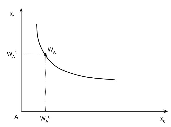
The trick of the Box is to rotate the indifference diagram for person $B$ so that their consumption is increasing in the down and left directions rather than the usual up-and-right direction:
Exhibit 53. Person B's Origin and Orientation
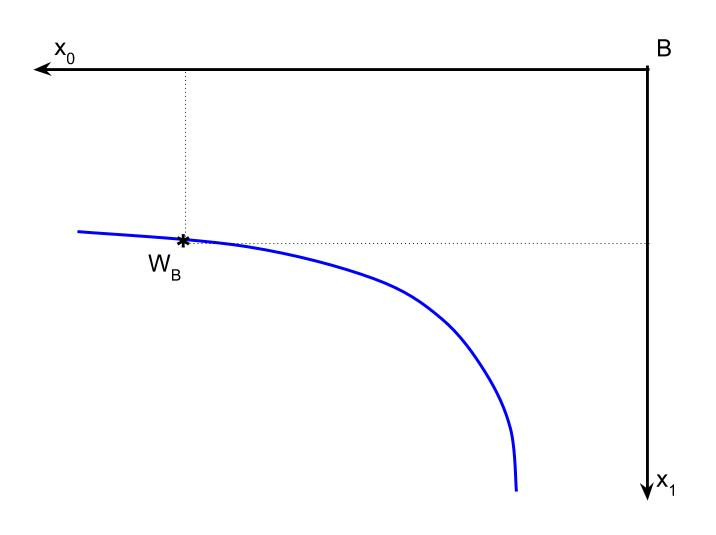
We want the box to include the total resource constraint as well as the individual endowments and preferences. The total resources in the economy is the vector sum of the endowments: $$W = W^A + W^B.\nonumber$$ If we visually think of moving B's graph onto the same graph as A we want $W^A$ and $W^B$ to be on top of each other. At that point B would consume their endowment and A would consume theirs. The width of the box is the total endowment of good 0. The height of the box is the total endowment of good 1.
Exhibit 54. An Edgeworth Box Combines A and B
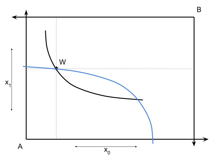
If there is no trade then person $i$ simply consumes $x^i = W^i$ and receives utility $U^i(W^i)$. However, gains from trade may allow both people to get more utility. A feasible allocation of the resources must satisfy the condition $x^A + x^B \le W$, and if we assume that everything is consumed we can simply require $x^A+x^B = W$. Any point in the box is feasible because measuring from the separate origins the total consumption vectors will always equal the total endowment.
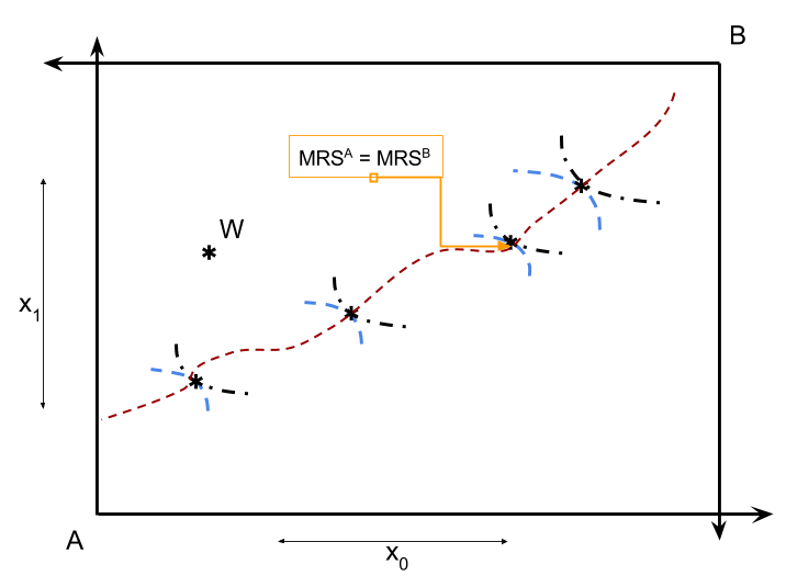
In general, a Pareto allocation is a feasible allocation for which neither person can be made better off without making the other worse off by changing to another feasible allocation. Let $\hat x^A$ and $\hat x^B$ be a Pareto allocation. With nice preferences, we can describe (an interior) Pareto allocation as one that satisfies a marginal condition. On the margin each person makes the same internal tradeoff between the two goods.
That is, A and B's MRSs are equal to each other at a Pareto allocation and all the resources are consumed: $$\eqalign{\hat x^B = W - \hat x^A\cr MRS^A\left(\hat x^A\right) = MRS^B\left(\hat x^B\right)\cr }\nonumber$$ We can combined the two conditions (efficiency and feasibility) into a single condition on $\hat x^A$: $$MRS^A\left(\hat x^A\right) = MRS^B\left(W - \hat x^A\right).\nonumber$$ Thus, the condition is a single non-linear equation with two free variables ($x^A_0$ and $x^A_1$). So in general there are many Pareto allocations.
Exhibit 55. Pareto Optimal Allocations
Of course, some of the allocations make one person worse off than if they did not trade and simply consumed their endowment. The closed region between the indifference curves that the individual endowment points lie on is called the core of the exchange economy. If A and B are willing to trade with each other they can consume at a point in the core and both are better off. We can call these feasible voluntary trades. Points that are in the core are defined as two inequalities in utility levels: $$\eqalign{U^A\left(x^A\right) &\ge U^A\left(W^A\right)\cr U^B\left(W-x^A\right) &\ge U^B\left(W^B\right)\cr}\nonumber$$
As with efficiency, the vector $x^A$ implicitly defines what B gets. Efficiency involves equalities of marginal utilities. Finally, a point on the contract curve combines both efficiency and voluntary trade.Exhibit 56. The Core and the Contract Curve
In reality we rarely trade face-to-face. Instead, we enter a market with prices with an amount of income and chose for ourselves. In this simple world, there are two prices: $(p^1,p^2)$, but we can normalize $p^1=1$ and focus on a single price. That is, we can think of good 1 and all other goods
and good 2 as some specific good we wish to focus on. The price of good 1 is 1 because allocations of it can be interpreted as dollars available to spend on other goods instead of good 2. So the price vector is $(1,p)$.
In a competitive market each person takes the price $p$ as given and makes an optimal choice subject to their budget constraint. Person A's budget constraint is: $$1x^A_0 + px^A_1 = 1W^A_0 + p W^A_1.\nonumber$$ Person B faces a similar budget constraint. If both people maximize utility subject to their budget constraint then each will satisfy their own individual marginal condition: $$MRS^i(x^i) = {p\over 1} = p.\nonumber$$ Note that this means that both MRS's will be equal to each other because they are both equal to the slope of the budget line. However, we can't lose track of the budget constraint. If person A satisfy it, then we add one more condition beyond the efficiency condition in a Pareto allocation: $\hat x^A_0 + p \hat x^A_1 = W^A_0 + p W^A_1.$ Note that this means that $\hat x^A_0$ is not free, its value is determined by $p$ and $x^A_1$: $$\hat x^A_0 = W^A_0 + p (W^A_1 - \hat x^A_1).\nonumber$$ Given that A consumes that much then B must in equilibrium consume what's leftover in good 0 endowment: $$\hat x^B_0 = W_0-\hat x^A_0 = W^B_0 + p(\hat x^A_1 -W^A_1).\nonumber$$
Thus a competitive allocation satisfies two equality conditions and has two free values to satisfy those constraints. Namely, we can set $p$ to a particular value, call it $p^\star$, and we can set $x^A_1$ to a particular value $\hat x^A_1$. The two conditions are then: $$\eqalign{ MRS^A\left( W^A_0 + p (W^A_1 - \hat x^A_1), \hat x^A_1 \right) &= p\cr MRS^B\left( W^B_0+ p (\hat x^A_1 -W^A_1), W^B_1+W^A_1 -\hat x^A_1 \right) &= p.\cr }\nonumber$$ We can write this as two equations that should be zero simultaneously. Simply subtract the price from both sides: $$\eqalign{ MRS^A\left( W^A_0 + p (W^A_1 - \hat x^A_1), \hat x^A_1 \right) - p &= 0\cr MRS^B\left( W^B_0 + p (\hat x^A_1 -W^A_1), W^B_1+W^A_1 -\hat x^A_1 \right) - p &=0\cr }\nonumber$$
Exhibit 57. A Competitive Equilibrium Allocation
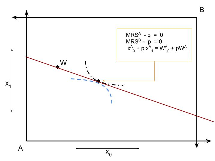
The two × two exchange economy is the simplest example of a competitive general equilibrium, and computational implementations are called computable general equilibrium (CGE). CGE analysis can be used to study the welfare effects of tax and transfer programs, gains from trade and other important policies. One solution strategy is to treat equilibrium prices as a system of simultaneous non-linear equations. We discuss the basic algorithms in section II. There are other iterative procedures as well. Judd 5.0; 5.10
Exercises
- Two utilities as functions.
- Two 2x1 endowment vectors
- A function that takes an allocation $x^A$ and returns a vector of MRS values at the point in the Edgeworth Box.
- Create a graph of the Edgeworth Box using graphics in Ox.
- Use Ox numerical tools to solve for Pareto allocations
- Use numerical tools to solve for competitive equilibrium.
- Generalize to $M$ goods.