- Basic Set up The hero of this section, Marshall, is a mild-mannered consumer from Detroit whose great-great-uncle was a British economist named Alfred. We consider how to model Marshall's consumption choices under different budget constraints. As usual we focus on two goods to illustrate the points, but having mastered numerical mathematical methods we can handle multi-dimensional problems as well.
- Set up the system of equations that describe an optimal bundle: the point where the MRS is tangent to budget line on the budget set: $$\eqalign{ MRS(x)\ &=\ p\cr p x_0+x_1 = m\cr}.\nonumber$$ Then solve the system of equations using the Newton-Raphson or Broyden algorithms discussed earlier.
- Since the budget is easy it can be used to solve for $x_1$ in terms of $x_0,$ $x_1=m-px_0,$ which results in a one-dimensional root that can be solved using Bracket-Bisect as well as Newton-Raphson. Obviously the bracket $[0,m/p]$ can be the first guess and bisecting can start right away.
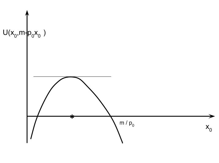
- Substitute for $x_1$ using the budget constraint and maximize the utility function over the value of $x_0$: $${\max}_{x_0}\ U(x_0,m-px_0)\nonumber$$ Then solve the unconstrained problem using one of the algorithms discussed earlier (e.g. BFGS or Nelder-Mead). Again, since it is a one-dimensional problem a Bracket-Bisect approach would work.
- Set up a constrained utility maximization (UM) problem and solve it using the SQP algorithm discussed earlier. In this case the budget would have to rewritten as $m -(p_0x_0+x_1) = 0$ so the constraint equals 0 on the budget line and is positive in the interior of the budget set. This is using a cannon to kill a fly but in higher dimensions with non-linear constraints a constrained optimization approach might be necessary.
- Multiple dimensions Now consider multi-dimensional consumption and price vectors: $$x = \pmatrix{x_0\cr x_1\cr \vdots\cr x_{N-1}}\qquad p = \pmatrix{p_0\cr p_1\cr \vdots\cr 1}.$$ We can still normalize the last price to 1. The equations that describe the demand vector are generalized. Instead of a single MRS condition there are $N-1$ conditions followed again by the budget equation: $$\eqalign{ {\partial U(x) / \partial x_0 \over \partial U(x) / \partial x_{N-1}}\ &=\ p_0\cr {\partial U(x) / \partial x_1 \over \partial U(x) / \partial x_{N-1}}\ &=\ p_1\cr \vdots\qquad &=\qquad \vdots\cr {\partial U(x) / \partial x_{N-2} \over \partial U(x) / \partial x_{N-1}}\ &=\ p_{N-2}\cr p\circ x &= m\cr }\tag{FOCn}$$ The budget can be written with vector notation. With a little more notation we can do the same with the tangency conditions. Define $\bar{y}$ as the first $N-1$ elements of a vector $y$: that is, simply chop off $y_{N-1}$. And define $\tilde{y}$ as the vector $y$ divided by the final element of $y.$ That is, $\tilde{y} = \bar{y}/y_{N-1}.$ Both of these new vectors have one less element than the original vector $y$: $$\overline{\pmatrix{y_0\cr y_1\cr\vdots\cr y_{N-2}\cr y_{N-1}}} \equiv \pmatrix{y_0\cr y_1\cr\vdots\cr y_{N-2}}\qquad \widetilde{\pmatrix{y_0\cr y_1\cr\vdots\cr y_{N-2}\cr y_{N-1}}} \equiv \pmatrix{y_0/y_{N-1}\cr y_1/y_{N-1}\cr\vdots\cr y_{N-2}/y_{N-1}} = \overline{y}/y_{N-1} $$ That looks complicated, but in Ox these "operators" are simple uses of vector indexing:
-
$\tilde{y}$ :
y[:rows(Y)-2]
$\bar{y}$ :y[:rows(Y)-2]/y[.last] - CES: Constant Elasticity of Substitution Utility Various utility functions are used in computational work. One of the most often used is the CES function. A simple version in two dimensions can be written $$U(x_0,x_1) = \left[ \alpha_0 x_0^\gamma + \alpha_1 x_1^\gamma \right]^{1\over\gamma}\nonumber$$ The parameters $\alpha_0$, $\alpha_1$ and $\gamma$ determine the rate of substitution between the goods (but when worked out the elasticity of substitution is a constant $1/(1-\gamma)$. The marginal utility ($U_i \equiv {\partial U\over \partial x_i}$) for good $i$ ($i=0,1$) is $$U_i = \alpha_i x_i^{\gamma-1}\left[ \alpha x_0^\gamma + \alpha_1x_1^\gamma \right]^{{1\over\gamma}-1}\nonumber$$ So the MRS simplifies to: $$MRS(x_0,x_1) = {\alpha_0\over\alpha_1}\left[{ x_0 \over x_1 }\right]^{\gamma-1}.$$ Notice that $\gamma\to 0$ the slope of the indifference curve becomes the same as the Cobb-Douglas utility function. And if $\gamma\to 1$ the slope becomes constant and we have linear utility. Finally, if $\gamma\to -\infty$ it can be shown that we get the Leontief utility $U(x_0,x_1) = \min\{x_0,x_1\}.$
//global parameters used by CES
decl  alpha,   // Nx1 vector of coefficients
         gamma;   // CES parameter

CES(x,aU,aS,aH)
   x  Nx1 vector of consumption
   aU CES Utility at x if defined
   return
        1 if defined
        0 otherwise

MRS(U,x)
    U  function U(x,aU,aS,aH) returning utility of consumption bundle x
    x  Nx1 vector of consumption

    return N-1 vector of Marginal Rates of Substitution for the utility
Note: - Solving the Consumer Problem as a System of Equations We could code a system of equations \eqref{UFOC} for $N$ values, the whole vector $x.$ Another approach is to use the fact that the budget is linear which makes it easy determine the value of one good using the budget line. Consider choosing just $\bar{x}$ (the first N-1 goods) and determine the final good as $$x_{N-1}(\bar{x}) = m - \bar{p} \circ \bar{x}.$$ This is a bit subtle. In the definition above we thought of $\bar{}$ as an operator on a vector. Now we are defining it as the vector we choosing of length $N-1.$ So nothing is being chopped off in that equation. If the consumer is spending more income on the first $N-1$ goods this will make the final good negative. So $\bar{x}$ is feasible if $x_{N-1}(\bar{x}) \ge 0.$ Otherwise it is infeasible and this cannot be a solution to the Marshallian demand. for the budget $(p,m)$. In fact, we also need to ensure that $\bar{x} \ge 0$ because a solution algorithm might wander off into negative territory.
ConsumerFOC(aFOC , xbar) aFOC address to return the system of equations for Marshallian demand xbar N-1 vector of free variables chosen (the final good determined by the budget line) Stored as globals prices, income, the utility function and utility parameters return 1 if system is defined at xbar 0 otherwise- Code a "package" to solve for Marshallian demand.
- Write a file
ConsumerFOC.oxhfile that declares the functionsMRS(),CES(),budget(),ConsumerFOC()and the global variables that they use. (The header file should also include the standard library and import the maximize and solvenle packages.) - Define the functions in
ConsumerFOC.oxusing the specifications above. - Write a a main program to test and use the function. It would look like:
#import "ConsumerFOC" main() { // initialize the global parameters (given separately) // call SolveNLE() // print out the demand vector and the indirect utility. } - Write a file
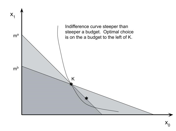
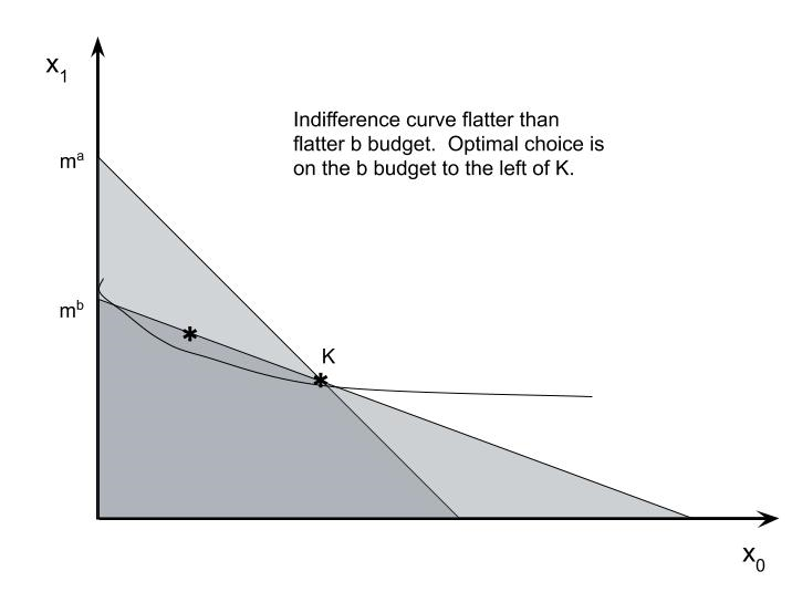
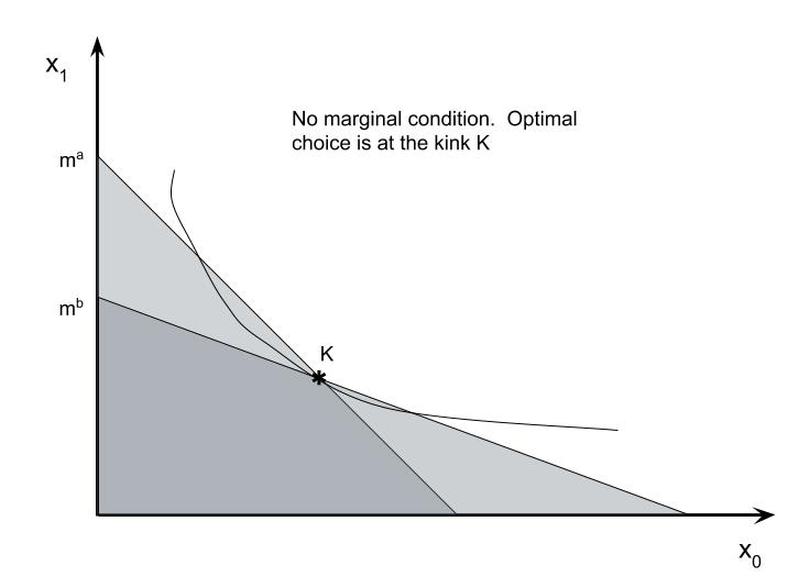
- Non-Linear Budget Sets Let's return to the two-dimensional version of Marshall, but now he faces a "kinked" budget set. In particular, there are two linear constraints:
- A: $\l(\matrix{p^a&1}\r) x \le m^a$
- B: $\l(\matrix{p^b&1}\r) x \le m^b$ NOTE: the price of good 1 is still normalized to 1. The price of good 0 is $p^a$ or $p^b$ depending on which constraint it is. The constraints satisfy two conditions (so the budget looks like the pictures below): $p^a > p^b$ and $p^am^b - p^bm^a$. There are two possibilities. Either Marshall's choice has to satisfy both budgets or it only has to satisfy one of them. If both constraints must be satisfied this means the budget is the dark shaded area in the pictures below. Notice that the budget set is a convex set in this case (a convex set has no holes or dents). On the other hand, if only one of the constraints has to be satisfied then the lighter regions are also affordable and the budget is not convex.
We start with a standard two-good problem, goods 0 and 1. We can let good 1 be a composite of all goods Marhall consumes other than good 0. Since good 1 is all goods other than good 2 we can think of $x_1$ as dollars (leftover to spend on other stuff). Let $x = (x_0,x_1)$ be the bundle consumed by Marshall an $U(x)$ is the utility of bundle $x$. We will keep the problem simple by assuming $U$ is strictly concave. $U()$ reflects the ordering of bundles: $U(x)> U(y)$ means $x$ is preferred to $y$. The utility numbers themselves do not matter.
If $U(x)=U(y)$ then we say that Marshall is indifferent between $x$ and $y$. The two bundles would appear on the same indifference curve. A single indifference curve is defined as the set of bundles that have equal utility: $$U(x) = {\bar U}\tag{IC}\label{IC}$$ where ${\bar U}$ is a number like 5 or -25.666788 or $\sqrt{\pi}$. In two dimensions a curve is a relationship between $x_1$ and $x_0$. The equation \eqref{IC} defines an implicit function: $$U\left( x_0,f\left(x_0;{\bar U}\right)\right) = {\bar U}.\nonumber$$ When we draw an indifference curve we are drawing $f(x_0;{\bar U})$ as a function of $x_0$. Different indifference curves come from different values of ${\bar U}$.
The slope of the indifference curve is the derivative of $f(x_0;{\bar U})$. We call the slope of $f()$ the marginal rate of substitution (MRS) between $x_0$ and $x_1$: $$MRS(x) \equiv f^{\,\prime}\left(\,x_0\,;\,U\l(\matrix{x_0\cr x_1}\r)\,\right) = -{\partial U(x) / \partial x_0 \over \partial U(x) / \partial x_1}.\tag{MRS}\label{MRS}$$
Marshall faces a budget constraint. The price of good 1 (dollars to spend on stuff other than good 0) can be normalized 1, so $p_1 \equiv 1$. The price of good 2 can be written $p_0$ but we can drop the subscript since the other price is normalized. Thus, Marshall's budget constraint is $$p x_0 + x_1 \le m.\tag{BC}$$ $m$ is Marshall's income. Notice it is in the same units as $x_1$ since $x_1$ is also dollars.
Marshall's problem is to maximize utility subject to the budget constraint. Let $x^{\star}(p,m)$ be a solution $$x^\star(p,m)\ =\ {\arg\max}_{p x_0+x_1\le m}\ U(x).\tag{Demand}\label{Demand}$$ To solve this problem numerically the form of the utility must be specified. Then we have several choices for solving this problem.
Exhibit 49. Consumer Demand As a System of Equations
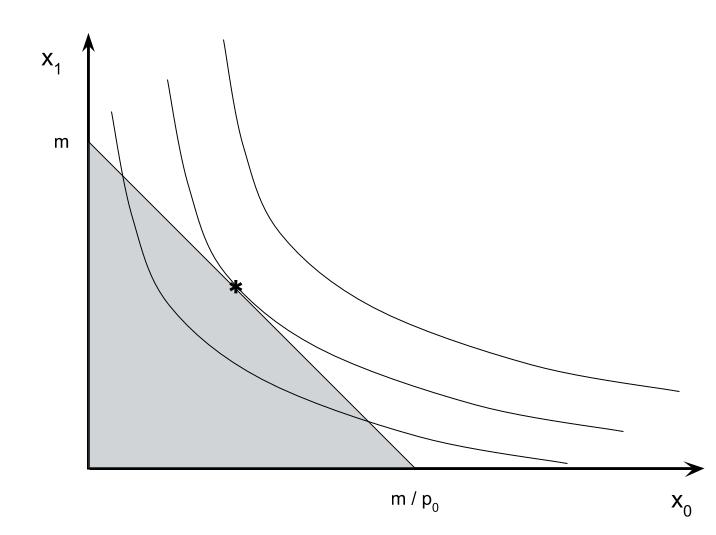
Exhibit 50. Consumer Demand As an Unconstrained Optimization Problem
With that notation we can define a vector version of MRS: $$MRS(x) \equiv {U_i \over U_{N-1}} \equiv {\widetilde {\nabla U(x)'}}.$$ (The partial derivatives are now denoted $U_i.$) The MRS vector is the gradient vector (transposed) divided by the final element of the gradient (and the last element chopped off). Then $\tilde{p}$ is the ratio of the prices to the final price (or simply $\bar{p}$ if it is normalized to 1).
The $N\times N$ system of equations that describe the Marshallian demand can be written $$ \eqalign{ MRS(x) - \tilde{p} &= \overrightarrow{0}\cr m - p\circ x &= 0\cr }\label{UFOC}\tag{UFOC}$$
For our purposes there is no need to limit the function to two goods. If $x$ is a $N\times 1$ vector then we can define the CES utility using vector and "element-by-element" operators: $$U(x) = \left ( \alpha \circ x^\gamma\right)^{1\over \gamma}.$$ Here $\alpha$ is a $N\times 1$ vector, so we can compute the sum as an inner product of $\alpha$ and $x^\gamma.$ The generalized $MRS(x)$ is then $$MRS(x) = \widetilde{ \alpha \circ x }^{\gamma -1}.$$ Again, the $\tilde{}$ means to take the ratio with respect to the last element of the vector and chop it off. Here is how you could code the general CES utility so that it is ready to be used by Ox's system solving and optimizing routines
MRS(U,x) can use the numeric gradient of any function $U()$ sent to it that is coded in the form required by Num1Derivative(). It is also possible to write a MRS routine specific to CES() using the analytic derivatives.
If we want to use SolveNLE() to find the optimal value of $\bar{x}$ we have to write a function that takes that as input and returns a $N-1$ system of equations. But our consumer(s) care about $N$ goods, so to compute utility and MRS we need to concatenate $x_{N-1}$ to $\bar{x}.$ One way to do this is to write a function that takes $\bar{x}$ and either returns the implied bundle on the budget line or some sort of error code if the bundle is not feasible. Let's call it budget(xbar):
decl  p,  //prices (the final price 1)
          m;      // income

budget(xbar,ax)
        xbar      on input N-1 x 1 vector of consumption
        ax        address, on return Nx1 vector of consumption on the budget line
                          xbar | x_(N-1)

        Stored as globals:
        p       N-1 x 1 price vector
        m       scalar income

        returns
                1 if x is feasible (all elements non-negative)
                0 otherwise
So budget() takes a N-1 vector and returns a N vector and a code to make it easy to check that the consumption bundle is feasible.
We have reduce the number of equations by 1 so that we get a $N-1 \times N-1$ system, but which is defined from the consumers utility that depends on $N$ goods:
$$MRS( B(\bar{x}) ) - \tilde{p} = \overrightarrow{0}.\tag{FOC}\label{FOC}$$
Here $B(\bar{x})$ just means equals the value returned in the address sent to budget(xbar,ax).
All these pieces come together for the function that defines the system of equations for the Marshall consumer problem in the form that can be sent to SolveNLE():
Exercises
The point where the two lines meet is the kink point marked $$K\ =\ (x_0^K,x_1^K) = \l(\matrix{ {m^a-m^b\over p^a-p^b} \cr {p^a m^b - p^b m^a\over p^a-p^b}}\r).\tag{Kink}$$ Bundle $K$ lies on both budgets. If you picture indifference curves of different slopes you might see that the optimal choice is partly determined by what happens at $K$. In particular, compute $|MRS(x)|$ at $x=K$. Define this slope as $MRS_K$.
If $MRS_K$ is larger than $p^a$ it means that the indifference curve is steeper than the slope of budget A. Then the optimal choice will be to the right of $K$. Whether it is on the A or B budget depends on whether Marshall must satisfy both or only one budget set. If it is both, the condition that describes optimal choice is $$MRS(x^\star_0,m^a-p^a x^\star_0) - p^a\ =\ 0.\nonumber$$ If only one budget set must be satisfied then use $p^b$ in the equation. On the other hand, if the MRS at $K$ is flatter than slope "b" budget ($p^b)$, then the optimal choice will be to the left of $K$. Now budget B is inside of A so $p^b$ would be used if both budgets must be satisfied.
Suppose $MRS_K$ is between $p^b$ and $p^a$: $p^b\lt MRS_K \lt p^a.$ That would mean that the indifference curve stays within the lightly shaded area of the graph. If both budgets have to be satisfied then the optimal choice will be at the kink, $x^\star = K$. There is no tangency condition. If the condition is either A or B then.
Exhibit 51. Kinked Budgets
