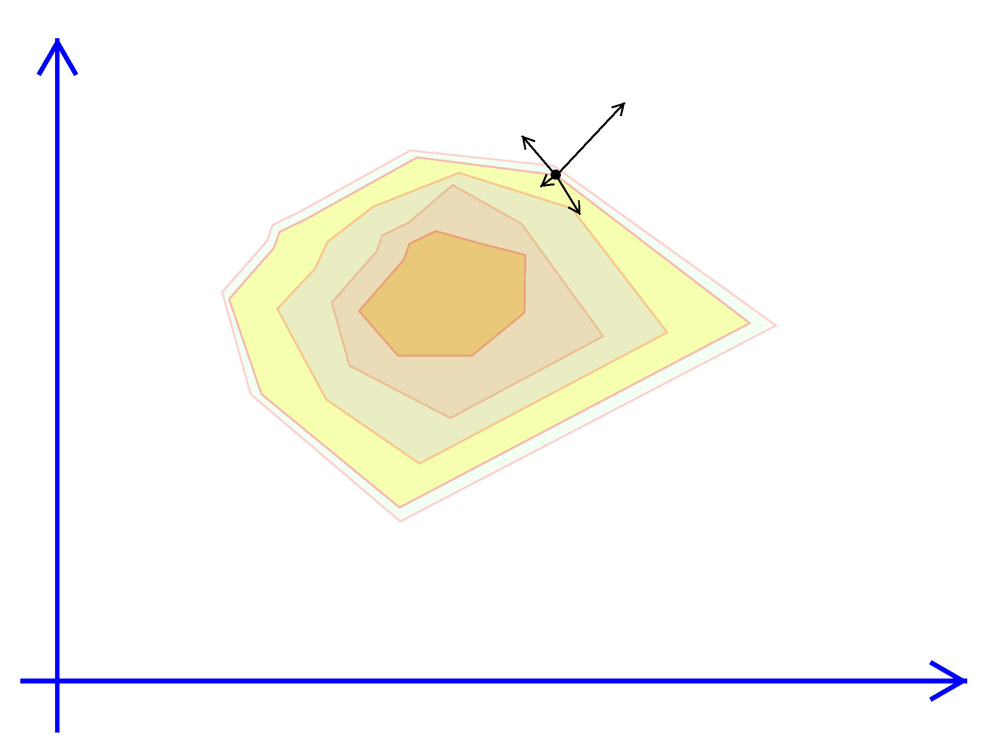
Exhibit 43. Gradients Do Not Help with Kinky Objectives

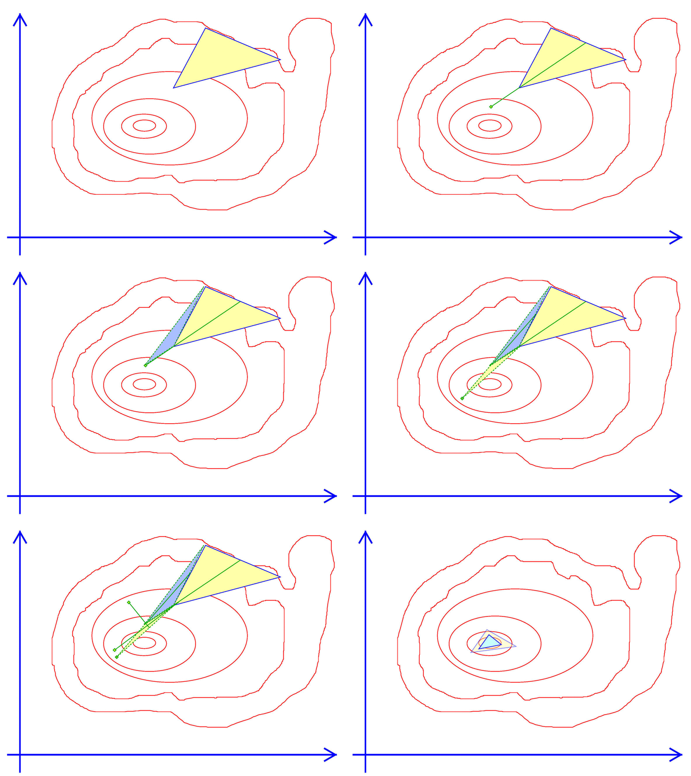
The basic algorithm creates a simplex which is a closed shape within the parameter space. If choosing one variable ($n=1$) then a simplex is simply an interval on the line. An interval is defined by its upper and lower limits, that is 2 points (or $2 = 1+1$) points. When choosing two variables ($n=2$) a simplex is a triangle, a shape that involves three (or $2+1$) vectors. For the triangle to have a non-zero area no two points or vertices can be on the same line. In general a simplex in $n$ dimensions is defined by $n+1$ points that are not co-linear.
Algorithm 18. The Nelder-Mead Amoeba Algorithm
- Initialization. Set $t=0$.
- Create a simplex in $\Re^n$ with $n$ other (not co-linear) points.
- Call these points $x^0, x^1, \dots, x^n$.
- ‡ Evaluate the objective at each vertex, $f^i = f(x^i)$. Identify the best ($f^M$), worst ($f^m$) and second worst ($f^s$) points.
- → Attempt A. Extend the best point. That is,
- Stretch the best vertex $x^M$ out further from all the other points (by a factor greater). Call it $x^A$.
- Evaluate the objective at that point, $f^A = f(x^A)$.
- Keep $x^A$ if is better than the current worst point.
- If $f^A \gt f^m$, replace $x^m$ with $x^A$. (Reset the values of $M,m,s$ to account for the change.) Return to → with the new simplex.
- If $f^A \lt f^m$ then go on to attempt B.
- Attempt B. Try moving away from worst point.
- That is, try $x^B$ which is on the opposite side of the simplex from $x^m$.
- If $f^B \gt f^m$ then keep it as in Attempt A an return to →.
- If not, try C.
- Attempt C. Collapse the simplex.
- Compute new points $x^0, \dots, x^n$ that are all a factor closer to the average point of the current Simplex.
- If the size of the new simplex is smaller than the precision $\epsilon$
 .
. - Otherwise, return to ‡ evaluate the objective at each point and identify M, m and s. Return to →.
Exhibit 44. Walk like an Amoeba

#import "maximize"

    MaxSimplex(func, ax, af, vDelta);

        Argument        Explanation
        ------------------------------------------------------------------------------------
        func            objective (in same form as other Max routines require)
        ax              address of starting values and where to place final values
        af              address to place final objective value
        vDelta          0 = initialize the simplex internally
                        n x 1 matrix of step sizes for the simplex

    Returns
        Convergence code same as MaxBFGS
Summary of Unconstrained Optimization
We started with the simplest problem: find a local maxima of a continuous function in one dimension using a line search, involving two steps: bracket then bisect. Then we generalized to finding a local maxima in any number of dimensions when the gradient (first derivatives) all exist everywhere (no kinks). Whether these gradient based algorithms converge depend on the shape and curvature of the objective. Then we added the Nelder-Mead routine which works well even if the function has kinks. Later we will add arandomsearch algorithm that tries to find a global maximum even when local maxima exist.
In practice, what algorithm should you use? The answer is, you should be prepared to use all of them, especially when maximizing a function of many parameters (large $n$) that you are not sure is concave and smooth (no kinks). In particular, you should see sequential optimization as a applying a sequence of algorithms from the most robust but inefficient to the fastest, typically Newton or BFGS. Typically you would monitor the progress of your algorithm. As the current best value stops changing quickly you can stop the algorithm and start the next one from where the last one left off.
Exercises
We can get back to the simple logit by setting J=2 and $\beta_0 = \overrightarrow{0}.$ That is option $0$ has beta vector of 0s, which means $e^{v_{i 0}} = e^{x_i\beta_0} = e^0 = 1.$ And now that function we've been working with all along becomes a special case of the multinomial logit log-likelihood function: $$L^J = \sum_{i=0}^{N-1} \ln \left( { e^{v_{i\,y_i}} \over \sum_{j=0}^{J-1} e^{v_{i\,j}} }\right),\qquad\hbox{and } v_{ij} \equiv x_i\beta_j.$$ Note that $L^J$ is shorthand. A more accurate definition would be $L^J(\beta_1,\dots,\beta_{J-1}; y, X).$ That is, $y$ and $X$ are taken as given. The vectors of coefficients are variable in order to maximize $L^J.$
In the simple logit we could maximize this function using Ox's MaxBFGS() by sending a single beta vector as the parameters to maximize over. In the multinomial model we want to maximize over 2 or more vectors, but MaxBFGS() like almost all optimizers takes only a column vector as the argument to maximize over. Let's define $\theta$ as that vector and think of it containing the "concatenation" of the $\beta_j$'s:
$$\theta \equiv \pmatrix{\beta_1\cr\beta_2\cr\vdots\cr\beta_{J-1}}$$
Note that we don't include $\beta_0$ because it is fixed at 0 and MaxBFGS() should not change its values. A function written to compute $L^J$ would "unpack" $\theta$ into a matrix:
$$\theta_{(J-1)K\times 1} \qquad \Rightarrow \qquad B_{K\times J} = \pmatrix{ \overrightarrow{0} & \beta_1 & \beta_2 & \cdots & \beta_{J-1}}.$$
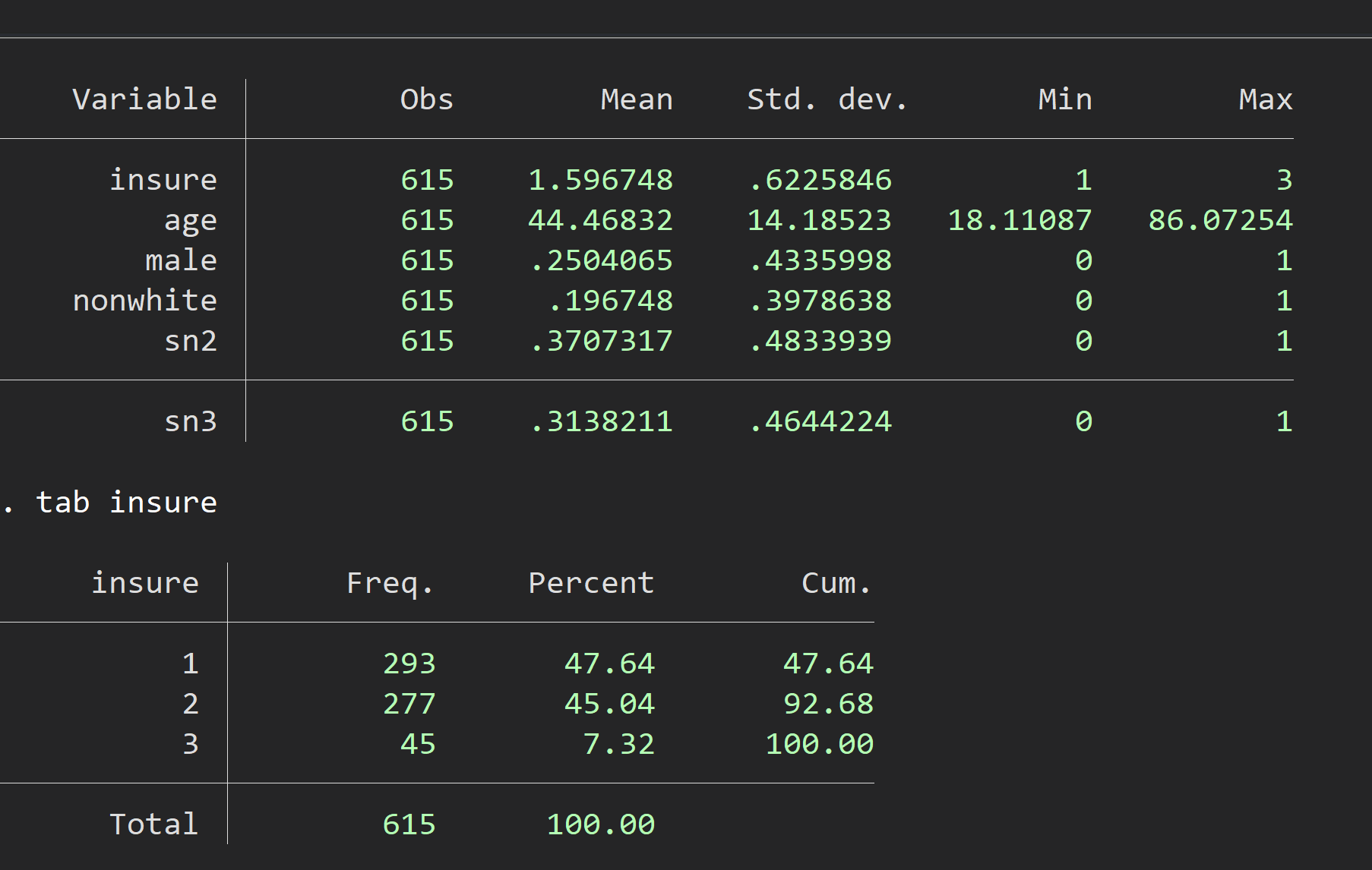
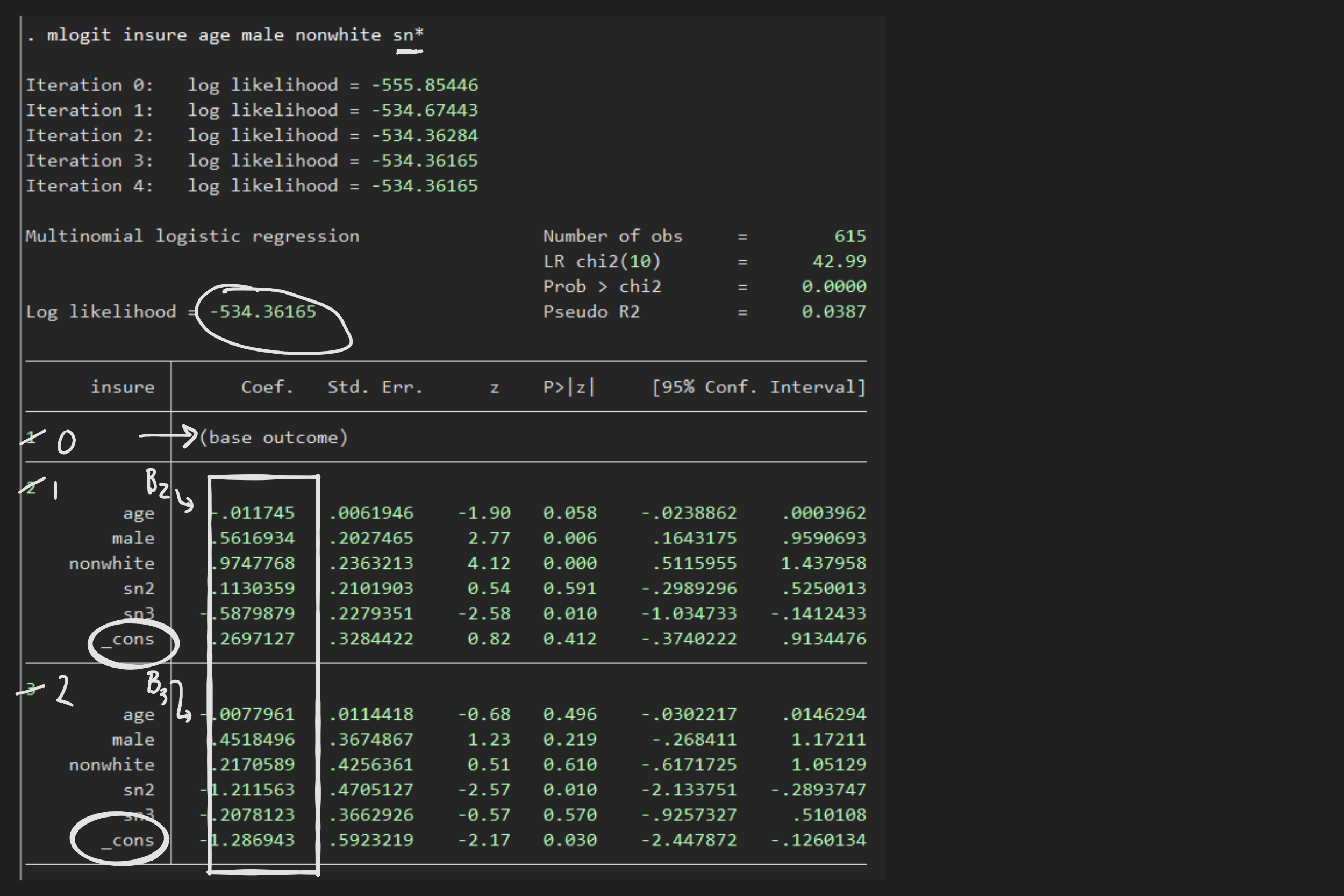
Now notice that $XB$ will contain a $N\times J$ matrix consisting of all the values $x_i\beta_j$ for all $i$ and all $j$. So computing $v_{ij}$ and ultimately $L^J$ can be done with vector functions (or with loops over $j$ or both $i$ and $j$). The code and data file in the mlogit folder is designed to build a function to compute $L^J$ and finding the maximizing coefficients using one of the Max????() algorithms. The data come from the example used in Stata to illustrate its mlogit command. The data and estimates are summarized with these screen captures:


Add code to the files in the folder to:
- Complete coding of LJ
- Create a starting theta vector
- Maximize LJ (use algorithm of your choice)
- Print out results to compare with Stata output
- EXTRA:
- copy over stata_logit_data.dta from the logit folder
- use of loaddemo to load the simple logit data data
- Reset K and J (*NOTE: do not decrement y since it is already 0/1)
- Verify LJ() to provides same results as simple logit