-
In more than one dimension the idea of bracketing a maximum becomes unworkable. Now we turn to calculus to help the algorithm decide which direction to go towards a maximum. That is, we use the partial derivatives (gradient vector) of the function to guide the search for improvement. In turns out that the line optimization technique of bracket-and-bisect still comes in handy.
- Steepest Ascent
- Given $f(x)$ and $x^0\in \Re^n$ and tolerance $\epsilon>0$.
- Initialize. Set $t=0$.
- →Compute Gradient. $\nabla\,f_t = \nabla\,f(x^t)$. Strong convergence: If $\|\nabla\,f_t\| \mathop{=_{\epsilon_1}} 0$, then
 .
. - Line Optimization. $$\lambda^\star = {\arg\max}_\lambda f\left(x^t + \lambda \nabla\,f^{\,\prime}_t \right).\nonumber$$
- Set $x^{t+1} = x^t + \lambda^\star\nabla\,f^{\,\prime}_t$.
- Increment $t$ and repeat previous two steps (go back to →).
- Set $t=0$. $\nabla\,f_t = \nabla\,f(x^t)$.
- Line Optimization. $\lambda^\star = {\arg\max}_\lambda f\left(x^t + \lambda \nabla\,f^{\,\prime}_t \right)$
- Set $x^1$.
- Line Optimization 2, etc.
- Two Examples Consider $$f(x_0,x_1) = -x_0^2 + x_0x_1 - x_1^2.\nonumber$$ As a quadratic function we get a linear gradient: $$\nabla\,f = (\,-2x_0+x_1\,,\,x_0 - 2x_1\,).\nonumber$$ First order conditions have a closed form solution, so it is easy to show that $x^\star = (0,0)$. If we started at $x^0 = (2,1)$, we have $\nabla\,f^0 = (-3,-1)$. It's easy to see that with a step size of $s^0=.75$ we get $$x^1 = x^0-(1.5)\nabla\,f^0 = (-0.25,.25).\nonumber$$ That might not be the exact line maximization step, but we can see get very close. It also turns out that once the current values are equal like that the symmetry of the gradient kicks in and the next step will hit $x^\star$ exactly (the reader is encouraged to verify or correct that claim). Therefore, Steepest Ascent works perfectly in two iterations! This is because the objective is quadratic so the Hessian is a constant matrix. That then means the gradient points in the right direction to go but it might not be the right length. Now consider a different simple function: $$f(x_0,x_1)=-\left(\,1-x_0\,\right)^{2}-100\left(\,x_1-x_0^2\,\right)^{2}.\tag{Rosenbrock}$$ This is known as the Rosenbrock function (see
- Newton's Method Newton's method is a big improvement over Steepest Ascent. It uses both the gradient vector and the Hessian matrix in order to speed up convergence to a maximum. Continuing with our mountain climbers in the fog analogy: rather than just going up the steepest path they would be better off thinking about how the gradient is changing within the area they can see. If they can see that the gradient is slowing down along the steepest path but stays steeper to one side of that path they would make quicker process if they
- Given $f(x)$, and $x_0\in \Re^n$ and tolerance $\epsilon_1$.
- Set $t=0$.
- →Compute $\nabla\,f_t$ Strong convergence: If $\|\,\nabla\,f_t\,\|\ \mathop{=_{\epsilon_1}}\ 0$, then
 .
. - Compute $H_t = Hf(\,x_t\,)$.
- Solve $H_t\,s_t = -\nabla\,f_t^T$ for the direction $s_t$.
- Perform line optimization on $\lambda$: $$\lambda^\star_t = {\arg\max}_\lambda f\left(x_t + \lambda s_t\right)\nonumber$$ Set $x_{t+1} = x_t + \lambda^\star s_t$.
- Increment $t$ and repeat previous two steps (go back to →).
- Quasi-Newton Methods
- Given $f(x)$, and $x_0\in \Re^n$.
- Initialize.
Compute $\nabla\, f_0$. Set $t=0$ and $H_0=I$ (or some other symmetric invertible matrix). - → Strong convergence: If $\|\,\nabla\,f_t\,\|\ \mathop{=_{\epsilon_1}}\ 0$, then
 .
. - Solve $H_t s_t = -\nabla\,f_t^T$.
- Perform line optimization on $\lambda$: $$\lambda^\star_t = {\arg\max}_\lambda f\left(x_t + \lambda s_t\right)\nonumber$$ Set $x_{t+1} = x_t - \lambda^\star_t$.
- Update $H$ (according to BFGS).
- Increment $t$ and repeat the previous 4 steps (go to →).
- Gradient-Based Methods in Ox
#import "maximize"

    MaxNewton(func, ax, af, aH, UseNH);

        Argument        Explanation
        ------------------------------------------------------------------------------------
        func            function that computes the objective (see format below)
        ax              address of starting vector, where final values will be placed
        aH              address to place final Hessian (can be 0 if not needed)
        UseNH           0=func computes Hessian
                        1=Use numerical Hessians computed in MaxNewton
        ------------------------------------------------------------------------------------

    Returns an integer Convergence Code:

          Value    Label            Explanation
        ------------------------------------------------------------------------------------------------
            0      MAX_CONV         Strong convergence Both convergence tests were passed
            1      MAX_WEAK_CONV    Weak convergence (no improvement in line search); step length
                                        too small but one test passed
            2      MAX_MAXIT        No convergence (maximum no of iterations reached)
            3      MAX_LINE_FAIL    No convergence (no improvement in line search); step length
                                        too small and convergence test not passed.
            4      MAX_FUNC_FAIL    No convergence (initial function evaluation failed)
            5      MAX_NOCONV       No convergence Probably not yet attempted to maximize.
        ------------------------------------------------------------------------------------------------
The function you write that you send to myobjective(x, af, agrad, aHess); Argument Explanation ------------------------------------------------------------------------------------ x parameter vector af address of where to put f(x) agrad address to place gradient 0 = gradient not needed aHess address to place Hessian 0 = Hessian not needed ------------------------------------------------------------------------------------ Returns 1: function computed successful at x 0: function evaluation failed at x
You should verify that this is a specialization of the function format required by if (!isint(agrad)) Num1Derivative(myobjective,x,agrad);
Note that "myobjective" is the name of your function, "x" is whatever you call the first formal argument and "agrad" is whatever you call the third formal argument.
27-maxnewton.ox
 1:    #include "oxstd.h"
 2:    #import "maximize"
 3:
 4:    const decl beta = 0.9;
 5:    f(x,af,ag,aH) {
 6:    	af[0] = -x[0]^2 + 0.5*x[0]*x[1] - x[1]^2 + beta*log(1+x[0]+x[1]);
 7:    	if (!isint(ag)) Num1Derivative(f,x,ag);
 8:    	return 1;
 9:    	}
10:
11:    main() {
12:    	decl xp = <2;1>, fv;
13:    	MaxControl(-1,1);
14:    	println("Conv. Code=",MaxNewton(f,&xp,&fv,0,0));
15:    	}
Output produced from the example above:
Starting values
parameters
       2.0000       1.0000
gradients
      -3.0000      0.00000
Initial function =                  -3

Position after 1 Newton iterations
Status: Strong convergence
parameters
  2.9771e-005  1.9326e-005
gradients
 -4.0216e-005 -8.8816e-006
function value = -7.53864179238e-010
Conv. Code=0
NR 10.6
Imagine you are hiking to the top of a mountain in a dense fog. You can't see the peak at all. All you can see is in which direction the terrain is going up, down or staying level at your feet. With nothing else to go on, you might as well climb in the direction where the terrain below your feet is steepest, hoping the pattern continues to the top. In addition, you are hiking with a friend and want to carry on a conversation. This means that you don't survey the terrain after every step. You head out in a direction and keep going for a while until you feel that you are no longer going up. Then you stop, look down again and move in the steepest direction again.
If that analogy makes sense then you understand the notion of steepest ascent broken down into steps (an algorithm!)
Algorithm 15. Steepest Ascent
Exhibit 40. Steepest Descent in Two Dimensions
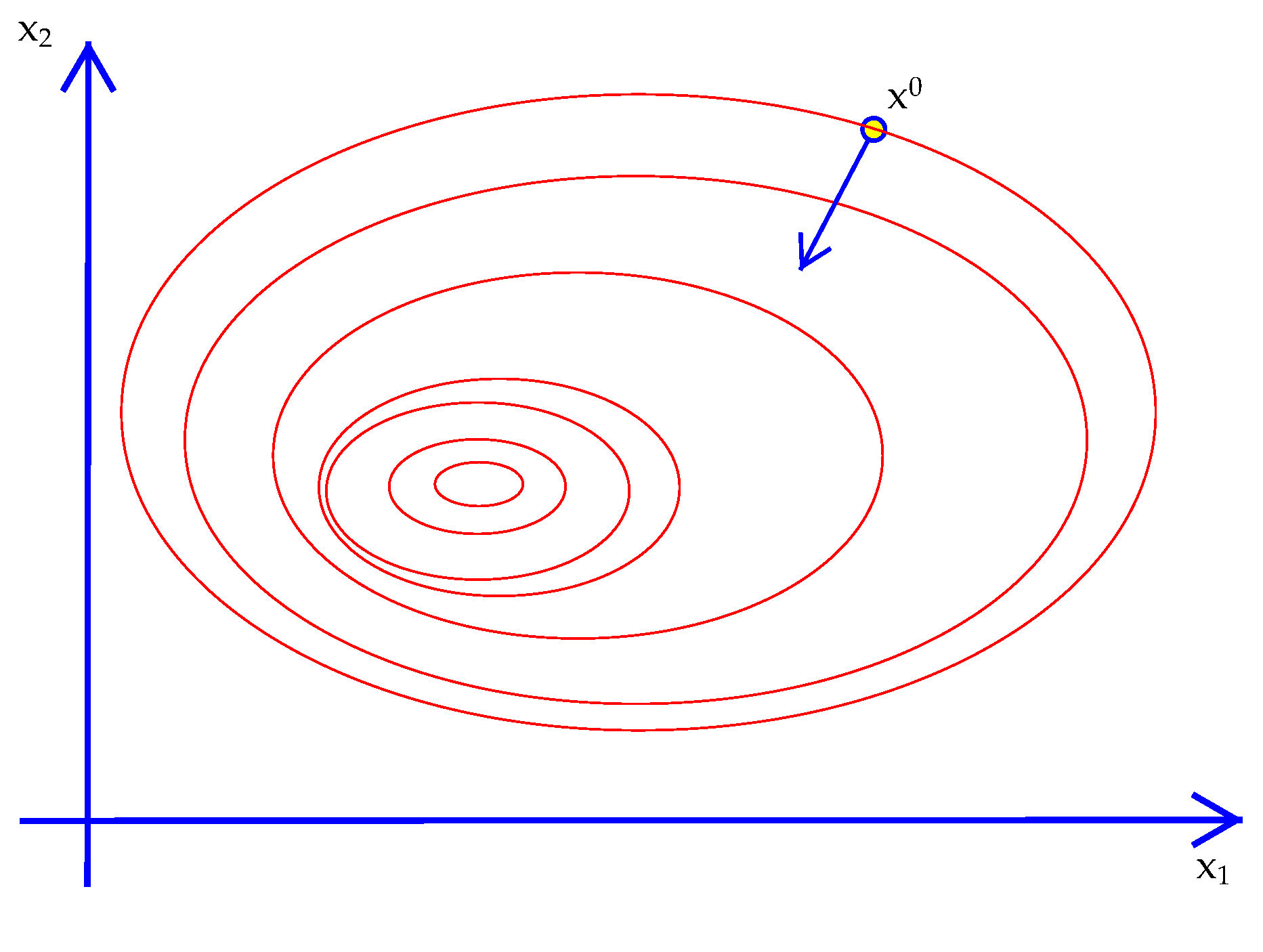
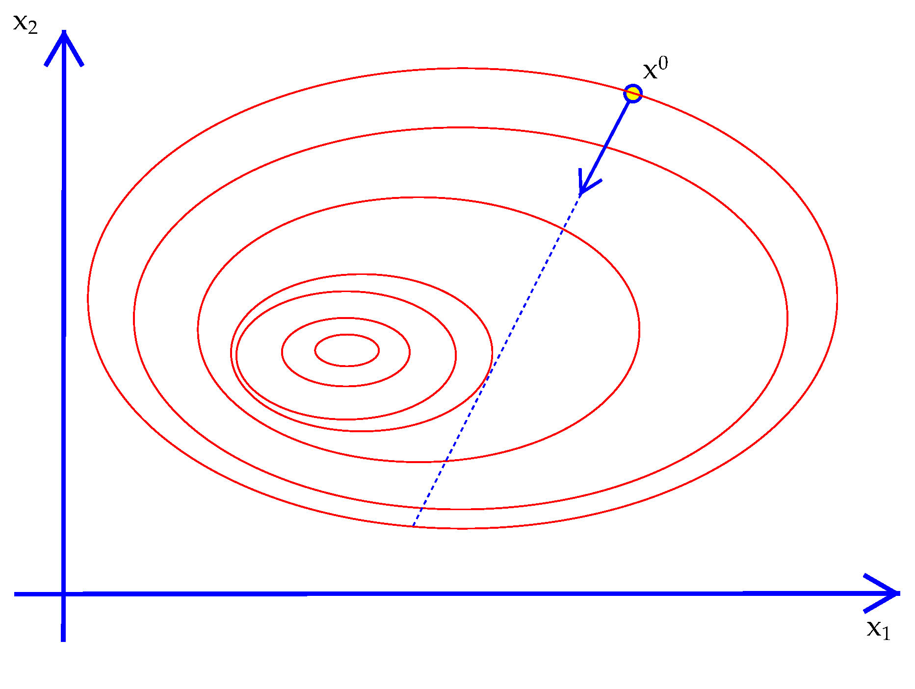

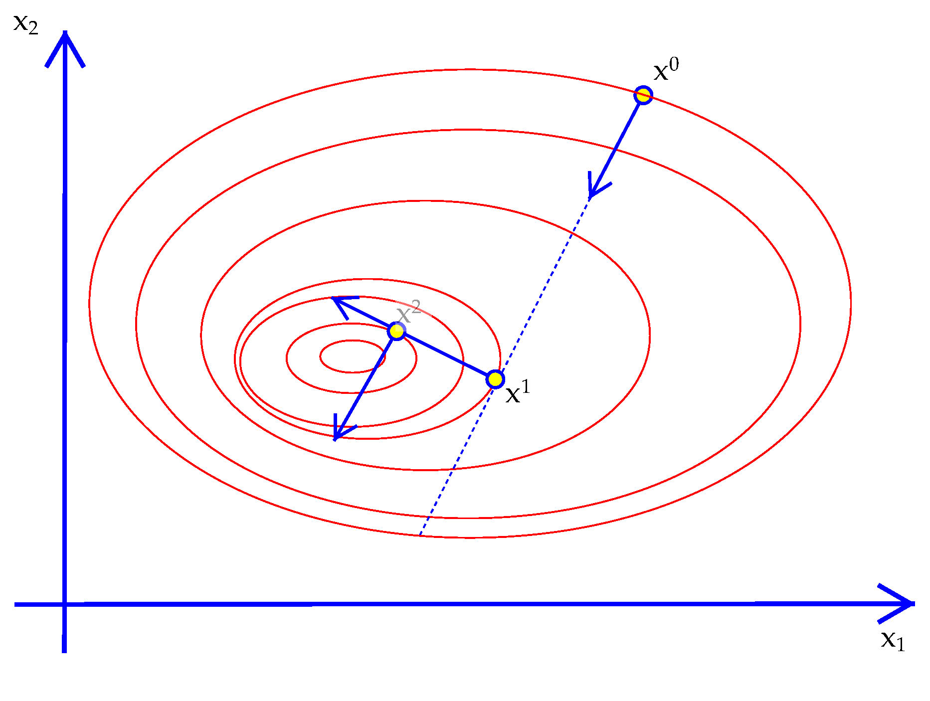
28-rosenbrock.ox). Again, $x^\star =(0,0)$. It turns out that Steepest Ascent cannot quickly find $x^\star$ as we will see later. The reason is that the gradient is almost never pointing in the direction of $x^\star$. Using information about how the gradient is changing will fix this problem, hence the value of using the Hessian as well as the gradient.
curledoff into that direction. The algorithm can be explained several different ways. One way is to use Taylor's second order approximation of any (smooth) function. Given the objective $f(x)$ and a point $x_0$ we compute the gradient vector and Hessian matrix at $x_0$, denoted $\nabla\,f_0$ and $Hf_0$. Then a Taylor approximation to the value of $f(x)$ at any point away from $x_0$ is $${f(x) \approx f(\,x_0\,) + (\,x-x_0\,)\nabla\,f_0^T + {1\over 2}\left(\,x-x_0\,\right)^T \left[ Hf_0\right] \left(\,x-x_0\,\right).}\tag{Taylor}\label{Taylor}$$ ($^T$ stands for the matrix transpose operator.) What is going is that the gradient and Hessian matrices at $x_0$ are determining a quadratic function on the right. Quadratic functions have closed form first order conditions and closed-form solutions to solving them. The max of the approximation would be $$x^\star = x_0 - H^{-1}f_0 \nabla\,f_0^T.\tag{QuadMax}\label{QuadMax}$$ However, our goal is not to maximize the approximation but rather to maximize the function itself. So $x^\star$ would be the true maximum only if $f(x)$ was actually quadratic (in which case the approximation is exact everywhere.). So Newton's method turns this closed form problem into an iterative process for the non-closed form original.
Algorithm 16. Newton Iteration
Exhibit 41. Newton versus Steepest Descent
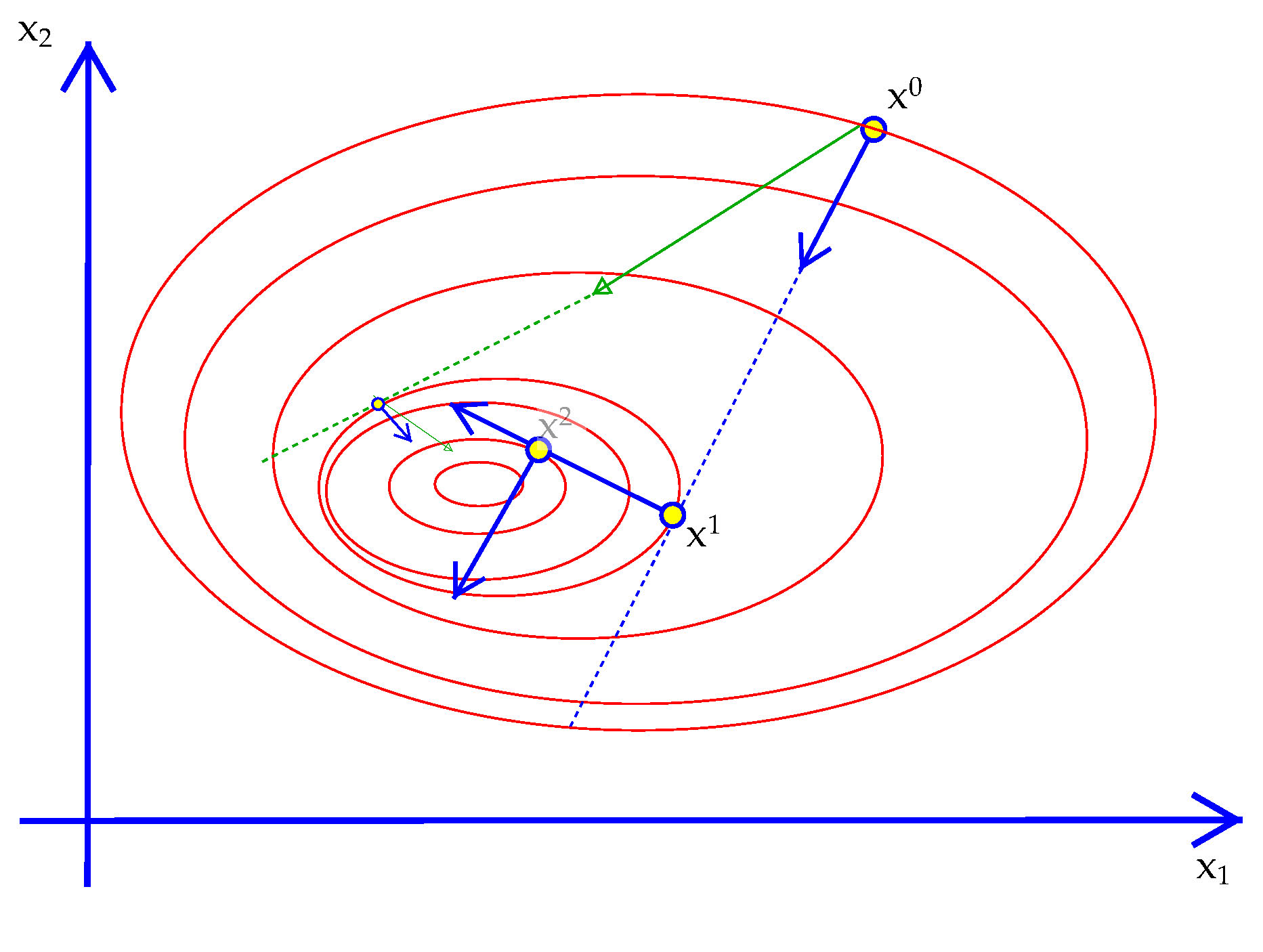
Exhibit 42. Newton and Bad Starting Values
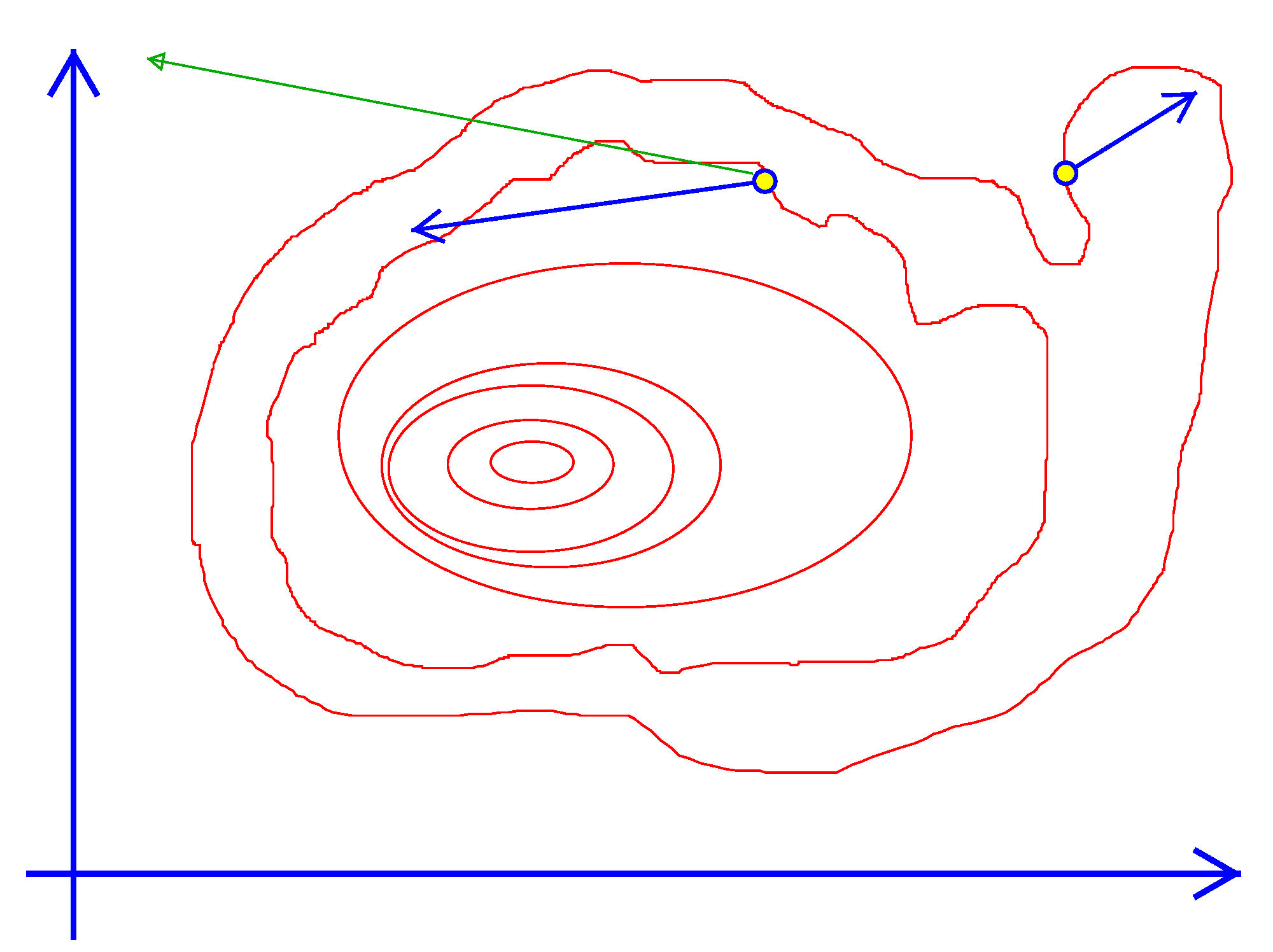
NR 10.7
A quasi-Newton algorithm uses the same step formula as Newton but it uses an approximation to the Hessian instead of computing it directly. Quasi-Newton algorithms build up the approximation to the Hessian as iteration proceeds. The formula uses the current Hessian approximation and the changes in the parameter vector and the gradient vector.
Different quasi-Newton methods are defined by different formulas for updating the Hessian approximation at each iteration. The formula that has become the standard is known as BFGS.
Algorithm 17. BFGS Updating
Compute $\nabla\,f(x_{t+1})$. Let $z=x_{t+1}-x_t$ and $y= \left(\nabla\, f_{t+1}-\nabla\, f_t\right)^T$.
BFGS Update: $${H_{t+1} = H_t - { (H_t z)(H_t z)^T\over z^TH_t z} + {yy^T \over y^T z}.}\tag{BFGS}\label{BFGS}$$
MaxNewton() has to be in a particular form since MaxNewton will call it.
Num1Derivative() and Num2Derivative(), which makes sense since they are all part of the maximize package. The difference is that the unspecified variable argument, …, is replaced by two specified arguments.
Notice that MaxNewton gives you the option of using numerical Hessians but your function must supply the gradient when asked for. That is, if the third argument agrad is not an int it is an address and it means that the algorithm wants the gradient computed as well as the function. But you can use Num1Derivative() rather than code the analytic derivatives. So if you want to send it to MaxNewton and don't want to code analytic derivatives add a line to your function that looks like this:
Recursion
This is an example of a recursive function call becausemyobjective() will be called within another call to myobjective(). Machinery in the background of the language keeps this from going terribly wrong. In particular, each call to a function goes on something called the "runtime stack" which keeps straight where the program is and which functions are still executing. Exercises
27-maxnewton.ox to a new file. Set beta=0 and modify it so that a new parameter alpha=0.5). Now set $\alpha = 1.999$ and then $\alpha = 2.0001$. Run the program to see how this affects the performance of Newton's method.28-rosenbrock.ox
1: #include "oxstd.h"
2: #import "maximize"
3:
4: decl fevcnt;
5:
6: rb(x,aF,aS,aH) {
7: aF[0] = -(1-x[0])^2 - 100*(x[1]-x[0]^2)^2;
8: if (!isint(aS)) Num1Derivative(rb,x,aS);
9: if (!isint(aH)) aH[0] = -unit(2);
10: ++fevcnt;
11: return 1;
12: }
13:
14: main() {
15: decl z = <1.5;-1.5>,frb,ccode;
16: rb(z,&frb,0,0);
17: MaxControl(-1,1);
18: fevcnt = 0;
19: // ccode=MaxNewton(rb,&z,&frb,0,1); //MaxBFGS Newton
20: ccode=MaxBFGS(rb,&z,&frb,0,1); //MaxBFGS Newton
21: println("x*=",z,"f(x*)=",frb,"/n convergence = ",ccode
22: ," #of eval: ",fevcnt);
23: }
24: