- Definition NR 4.0, 4.1
KC 14.3
Judd II.7
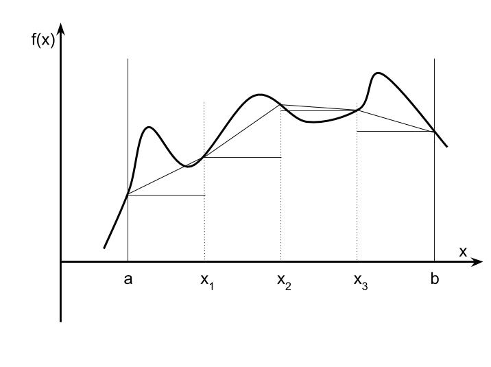
The intuitive notion of an integral is - A finite Riemann sum based on rectangles:
- Split the range $[a,b]$ in two and calculate the area of two rectangles:
$${\hat R}_1 = {1\over 2(b-a)}f\l( a+{(b-a)\over 2} \r) + {1\over 2(b-a)}f(b) = {1\over b-a}\left[ {1\over 2}f( a+{(b-a)\over 2} ) + {1\over 2}f\left(a+{2\over 2}(b-a)\right)\right]$$
- That is a rough calculation for the area under the curve $f(x).$ Notice it can be written as the inverse of the range $1/(b-a)$ times a weighted sum of two function evaluations where the weights add up to 2. If we split each one into two we get an approximation based on four points we can write this 3 different ways: $$\eqalign{ {\hat R}_1 &= {1\over 4(b-a)}f\l(a + {1(b-a)\over 4} \r) + {1\over 4(b-a)}f\l(a + 2{(b-a)\over 4} \r) + {1\over 4(b-a)}f\l(a + {3(b-a)\over 4} \r) + {1\over 4(b-a)}f\l(a + {4(b-a)\over 4} \r)\cr &= {1\over (b-a)}\l[ {1\over 4}+f\l(a + {1(b-a)\over 4} \r) + f\l(a + {3(b-a)\over 4} \r)\r] + {1\over 2}{\hat R}_1\cr &= {1\over b-a}\l[ {1\over 4}\sum_{i=1}^4 f\l(a + {i(b-a)\over 4} \r) \r].\cr } $$ So the second way shows that we can "iterate" on previous approximations. Each new level of integration would split the previous rectangles in two and evaluate the function in the midpoints. These new points would be weighted and added to half of the previous total. (That is, we could go to 8 points, 16 points, \dots, computing 4, 8, \dots new function evaluations.) That means we could keep going until the sum stops changing much (converges with some tolerance): stop at $k$ when $\|{\hat R}_{k+1}-{\hat R}_k\| \lt \epsilon.$ Or, the third version simply says to compute 4 points and weigh them with weights that add to one. In general, we could fix the number of points to evaluate, $n$, and use that as approximation. We would not be controlling the error compared to the true $\int_a^b f(x)dx$ but if this integral enters other calculations the error may not be that important. This is the same as the idea that we compute a numerical derivative using only two function evaluations. We could get a better approximation to the tangent if we computed more points, but it is rarely worth it. In the case of integration, we certainly don't want to stop at $n=2,$ but we may not worry about iterating in a loop until the change is less than $\epsilon.$ Once the bigger problem is complete we could go back and increase $n$ and see if it matters to the final result.
In the case of rectangles we never use $f(a).$ A better approximation adds a triangle on top of a rectangle and computes areas of trapezoids:
- That is a rough calculation for the area under the curve $f(x).$ Notice it can be written as the inverse of the range $1/(b-a)$ times a weighted sum of two function evaluations where the weights add up to 2. If we split each one into two we get an approximation based on four points we can write this 3 different ways: $$\eqalign{ {\hat R}_1 &= {1\over 4(b-a)}f\l(a + {1(b-a)\over 4} \r) + {1\over 4(b-a)}f\l(a + 2{(b-a)\over 4} \r) + {1\over 4(b-a)}f\l(a + {3(b-a)\over 4} \r) + {1\over 4(b-a)}f\l(a + {4(b-a)\over 4} \r)\cr &= {1\over (b-a)}\l[ {1\over 4}+f\l(a + {1(b-a)\over 4} \r) + f\l(a + {3(b-a)\over 4} \r)\r] + {1\over 2}{\hat R}_1\cr &= {1\over b-a}\l[ {1\over 4}\sum_{i=1}^4 f\l(a + {i(b-a)\over 4} \r) \r].\cr } $$ So the second way shows that we can "iterate" on previous approximations. Each new level of integration would split the previous rectangles in two and evaluate the function in the midpoints. These new points would be weighted and added to half of the previous total. (That is, we could go to 8 points, 16 points, \dots, computing 4, 8, \dots new function evaluations.) That means we could keep going until the sum stops changing much (converges with some tolerance): stop at $k$ when $\|{\hat R}_{k+1}-{\hat R}_k\| \lt \epsilon.$ Or, the third version simply says to compute 4 points and weigh them with weights that add to one. In general, we could fix the number of points to evaluate, $n$, and use that as approximation. We would not be controlling the error compared to the true $\int_a^b f(x)dx$ but if this integral enters other calculations the error may not be that important. This is the same as the idea that we compute a numerical derivative using only two function evaluations. We could get a better approximation to the tangent if we computed more points, but it is rarely worth it. In the case of integration, we certainly don't want to stop at $n=2,$ but we may not worry about iterating in a loop until the change is less than $\epsilon.$ Once the bigger problem is complete we could go back and increase $n$ and see if it matters to the final result.
- A finite Riemann sum based on trapezoids:
- $${\hat R}_n = {\sum_{i=0}^{n-1}} {b-a\over n}\left( f\left(a+i(b-a)/n\right) + {1\over 2}\left(f\left(a+(i+1)(b-a)/n\right)-f\left(a+i/n\right) \right) \right).\tag{Riemann}\label{Riemann}$$
- $n$ function evaluations, $n-1$ rectangles below $n-1$ triangles. With a little rearranging, it is possible to see that this too can be written as an iterative procedure.
- For $n=1$: $\hat R_1 = (b-a)\left[ {1\over 2} f(a) + {1\over 2} f(b) \right] $
For $n=2$: $\hat R = (b-a)\left[ {1\over 4} f(a) + {1\over 2} f\left(\left(a+b\right)/2\right) + {1\over 4} f(b) \right] = {1\over 2}R_1 + {1\over 2}f\left(\left(a+b\right)/2\right)$ - In general $${\hat R_n = (b-a) {\sum_{i=0}^{n-1}} \omega^i_n f(x_i)\ \hbox{and} {\sum} \omega_i = 1.}\nonumber$$
- Different sets of weights are designed to reduce the error between $\hat R$ and $S$. Weights include Trapezoid, Simpson, and Romberg formulas.
- Iterative integration: $R_n = {1\over 2}R_{n-1} + {1\over 2}\sum_{i=1}^{n/2} f\left(x_{2i-1}\right)$ Start at $n=1$ and proceed until $|R_n-R_{n-1}| \lt \epsilon$. A bad idea in a vector/interpreted language or under parallel execution.
- Or: fix the depth $n$ and compute all at once. Later check sensitivity of results by increasing $n$.
- Improper Integrals NR 4.3
KC 14.4 - $S=\int_a^b f(x) dx$, where $f(a)$ or $f(b)$ undefined, including the possibility that $a=-\infty$ or $b=\infty$. If the interval is unbounded (say, $b=\infty$) then for $S$ to exist $\lim_{x\to \infty} f(x)=0$.
- Change of variables: $z = g(x)$, $g$ monotonic and differentiable, $\left[g^{-1}\left(a\right),g^{-1}(b)\right]$ is compact. Then $$S = \int_a^b f(x)dx = \int_{g^{-1}(a)}^{g^{-1}(b)} f(g(z)) |g^{\,\prime}(z)| dz\tag{Improper}\label{Improper}$$ So apply the transformation and use a technique for proper integrals.
- Gaussian Quadratures NR 4.5
Error in approximating $S$ can be reduced for a given number of evaluations by choosing weights and nodes together for integrands of particular form that use orthogonal polynomial approximation to the function $f(x)$. Let $\{ (x_i,\omega_i) \}_{i=1,\dots,n}$ be a set of nodes (or points to evaluate at) and weights. In the rectangle and trapezoid formulas above the nodes are equally space over the range $(a,b).$ But in the case of Gaussian Quadratures the nodes are not evenly spaced. Furthermore, for reasons that may be clearer later, the integration consider by GQ is "weighted" by a function $g(x).$ This is not to be confused with the weights $\omega_i$ although there is a definite connection between the two. So problem is to approximate an integral of the form
$${S = \int_a^b f(x) g(x) dx \approx {\sum_{i=1}^n} \omega_i f(x_i) = S^\star.}\tag{GQ}\label{GQ}$$
Note that $g(x)$ does not appear in the weighted sum: its effect is built into $g(x)$.
The key things to keep straight about using GQs is that $\{ (x_i,\omega_i) \}_{i=1,\dots,n}$ depend jointly on the range of integration $(a,b)$ and the weighing function $g(x).$ Often you just want to integrate a function $f(x)$ and no "weighting function" is involved. That does not stop you from using GQ. If your integrand does not factor into a $g(x)$ of one of the common forms, rewrite it as ${f(x)\over g(x)}g(x).$ Now you can apply the GQ formulas that apply to the $g(x)$ to your modified integrand $f(x)/g(x)$.
the area under a curvewhich is correct for one-dimensional integral of a positive function. We write $\int_a^b f(x)dx$ as the integral of $f(x)$ from $a$ to $b$. As a calculus concept the integral is a limit of a process, in this case the limit of a sum.
Exhibit 36. Riemann Sums

Algorithm 8. Newton-Cotes Approximations to $S$
Algorithm 9. Numerical Approximation to Improper Integrals
Second, if you want to integrate over a range that does not match the one for the particular GQ formula you have transform your area of integration to match exactly the $(a,b)$ specified. This is less complicated than it sounds as we'll see when looking at the common ones used in economics.
The key theoretical result for GQ is that if the integrand is a polynomial of degree $2n-1$ then the approximation using $n$ nodes is exact. Thus, for a function that is well-approximated by, say, a 19th order polynomial using only $n=10$ points will be very accurate, especially when compared to the equal-spaced Newton-Cotes formulas.
Algorithm 10. Gaussian Quadrature Names and Ranges
| Name | Weight $g(x)$ | Interval | Coverage | Transformation |
|---|---|---|---|---|
| Gauss-Legendre | $1$ | [-1,1] | Any proper integral $f(y)$ over $[a,b]$ | $x_i=-1 + 2(y_i-a)/(b-a)$ |
| Gauss-Chebyshev | ${1\over \sqrt{1-x^2}}$ | |||
| Gauss-Hermite | $e^{-x^2}$ | $(-\infty,\infty)$ | Double unbounded integral $f(y)$ (often normal expectation) |
$x_i=(y_i-\mu)/\sqrt{2\sigma^2}$ |
| Gauss-Laguerre | $e^{-x}$ | $(0,+\infty)$ | Any half-plane (continuous discounting with $r$) |
$x_i=r(y_i-a)$ |
#includeSuppose you want to integrate $f(x)$ over $[a,b],$ and the function is defined everywhere in that range. Then code $f(x)$ as a simple functionQNG (func, a, b, aresult, aabserr);
f(x) which returns the value. (The QuadPack functions do not require your function to return the value through an address, but if you call the wrong function for the problem it won't work.) Then send it as QNG(f,a,b,&S,&err). A return value will explain the result (a value of 0 means the approximation was successful.). The result will be returned in S and a measure of error returned in err.
Suppose $f(x) = 1/x$ and you want to integrate over $[1,2].$ Then QNG() works fine. But suppose you want to integrate over $(0,1].$ Now, the integrand equals $\infty$ at the endpoint and the area under the curve is actually infinite as well. QNG() will not work which is good because the integral is undefined. It will try but it will return an error and S. Some of the routines in QuadPack will handle functions with singularities, but we'll focus on the more common case of an improper integral such as over the range $(a,\infty), $(-\infty,b)$, or $(-\infty,+\infty).$ All of these cases are handled with
QAGI(func, bound, inf, aresult,aabserr);

Interval        bound           inf
(a,∞)            a                1
(-∞,b)           b               -1
(-∞,+∞)          0               -2
So, suppose you want to integrate $f(x) = e^{-x}$ from $(2,+\infty).$ Then
QAGI( f,2.0,1,&S,&err) will do it.
        0: normal and reliable termination of routine;
        1: maximum number of steps has been executed;
        2: roundoff error prevents reaching the desired tolerance;
        3: extremely bad integrand behaviour prevents reaching tolerance;
        4: algorithm does not converge;
        5: integral is probably convergent or slowly divergent;
        6: invalid input;
       10: not enough memory;
See the QuadPack Package documentations for other functions to handle other cases.
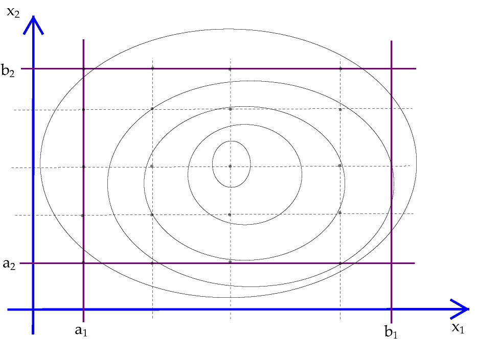
Exhibit 37. Two Dimensional Integral
