- Probability and Random Variables: a Review A random experiment is a process leading to two or more possible outcomes, with uncertainty as to which outcome will occur. For example, rolling a die or flipping a coin are random experiments. If we list or describe every possible outcome that might occur in a random experiment we call that the sample space. To be complete, the sample space is not just the set of all outcomes; it also includes the probability that each outcome will appear in a random experiment. The easiest case is when each outcome is equally likely (like rolling a die or flipping a fair coin). But cases where outcomes are not equally likely are also easy to imagine. In words, a random variable is a numerical value associated with the outcome of a random experiment. A way to visualize the random variable is as the column on the sheet of paper or the spreadsheet used to record values associated with an experiment. We distinguish between two types of random variables, discrete and continuous. Another useful way to think of a random variable is the collection of possible measurements. Once a random event happens the value of the random variable is realized. Based on its definition a random variable is neither random nor a variable. It is a deterministic function of something that is random (the outcome). What is random and variable is the realized value the random variable takes on in a particular experiment. A discrete random variable takes on only a finite number of different values with positive probability. That is, if $Y$ is discrete then $P(Y=y)\gt 0$ only if $y \in \{y^1,y^2,\dots,y^M\}$. A continuous random variable can take on any value in one or more intervals of the real line. A (pure) continuous random variable takes on no particular value with positive probability. The cumulative distribution function (cdf) $F(y)=Prob(Y\le y)$. of a random variable $Y$ is the probability that $Y$ is below a given value. We often use $F(y)$ to denote the cdf. We relate the cdf to probability as: $$F(y) \equiv Prob( Y\le y).\nonumber$$ We write $Y\quad \sim\quad F(y)$ to mean $Y$ is a random variable with cdf $F(y)$. The cdf is just a way to summarize how the probability of events determines the pattern of a thing we can measure from an experiment. There are other ways to summarize this information. One reason not to start with the cdf is that it is not really the way most people's brain would visualize uncertain outcomes. The reason to start with the cdf is that the definition is the same for discrete and continuous random variables. However, because of those technical issues we are trying to avoid, we have to make a slight distinction between kinds of random variables when talking about the more intuitive notion of probability or density function.
- Joint Probability and Distribution Let $A$ and $B$ be two events. $P(A,B)$ is the probability of A and B jointly occurring in the same random experiment: $$P(A,B) \equiv P( A \cap B).\nonumber$$ The definition says that "joint" is like intersecting two sets, because the joint probability of two events is the probability that both happen in the same random experiment. If in the abstract view events are sets then joint means the outcome is in both events, hence intersection is called for. Now suppose $Y_1$ and $Y_2$ are two random variables defined on a sample space with probability $P()$. The the joint cumulative distribution function (joint cdf) of two or more random variables is the bivariate function that gives the probability that both are below certain values: $$\hbox{for all } y_1, y_2,\quad F(y_1,y_2) \equiv Prob( Y_1\le y_1, Y_2\le y_2).\nonumber$$ The joint pdf for discrete random variables is the bivariate function giving the probability the random variables equal certain values: $$\hbox{for all }y_1, y_2,\quad f(y_1,y_2) \equiv Prob( Y_1= y_1, Y_2= y_2).$$ The joint pdf for continuous random variables is the bivariate function giving the rate of change in the cdf: $$\hbox{for all }y_1, y_2,\quad f(y_1,y_2) \equiv {\partial^2 Prob( Y_1= y_1, Y_2= y_2)\over \partial y_1\partial y_2} = {\partial^2 F(y_1,y_2) \over \partial y_1\partial y_2}.$$
- Let $Y_1$ and $Y_2$ be two random variables with joint cdf and pdf $F(y_1,y_2)$ and $f(y_1,y_2)$.
- If $Y_2$ is discrete and takes on $M$ different values, denoted $y^1_2,\dots,y^{M}_2$, then the marginal cdf of $Y_1$ is $$F_1(y_1) = Prob(Y_1\le y_1) = F(y_1,y_2^{M}).$$ If $Y_1$ is discrete the marginal pdf of $Y_1$ is $$f_1(y_1) = Prob(Y_1 = y_1) = {\sum_{k=1}^{M}}f(y_1,y^k_2).$$
- If $Y_2$ is continuous then the marginal cdf of $Y_1$ is $$F_1(y_1) = Prob(Y_1\le y_1) = F(y_1,\infty).$$
- If $Y_1$ is continuous then its marginal pdf is $$f_1(y_1) = {d Prob(Y_1 = y_1)\over dy_1 }= \int_{-\infty}^{+\infty}\ f(y_1,y_2)dy_2.$$
- Some Distributions The simplest possible continuous distribution is the standard uniform, sometimes denoted $U(0,1)$. We write $V\sim U(0,1)$ to mean
- $V$ is a continuous random variable that takes values strictly between 0 and 1.
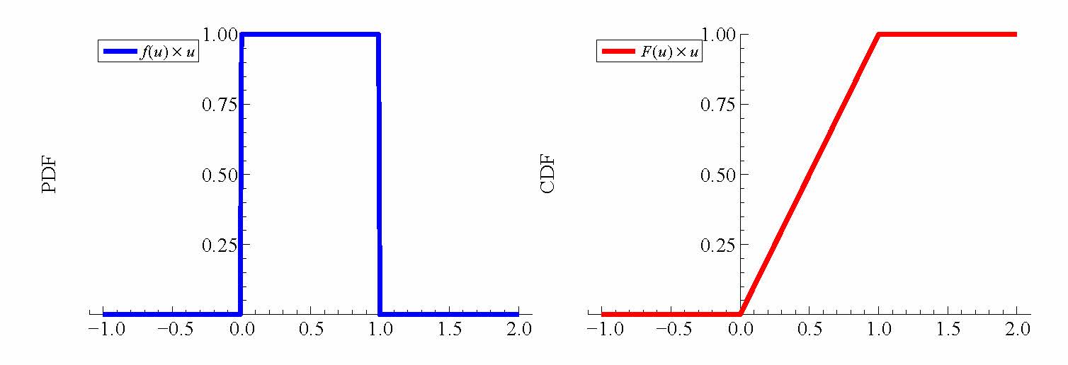
- $V$ has a uniform (constant) pdf on (0,1). To make the total probability integrate to 1 the height of the density is 1:
- $f(v) = \cases{ 1 & for $0\le v\le 1$\cr0 & otherwise\cr}$
- The cdf of $V=\int_{0}^{v}f(u)du$ is simply $v$:
- $F(v) = \cases{ 0 & for $v\le0$\cr v & if $0\lt v \lt 1$\cr 1 &if $v\gt 1$}$
- $Z$ is a continuous random variable that takes on values between $(-\infty,+\infty)$.
- The pdf of a Z variable is usually denoted $\phi$ and equals $$\phi(z) = {1\over\sqrt{2\pi}}e^{-z^2/2}.\nonumber$$
- The CDF of a $Z$ random variable is denoted $\Phi$ and equals $$\Phi(z)= \int_{-\infty}^z \phi(v)dv.\nonumber$$ This integral has no closed form expression. This is the reason stats books contain tables of normal values.
- $X$ is a continuous random variable that takes on values between $(-\infty,+\infty)$.
- It has pdf of the form $$f(x) = {1\over\sqrt{2\sigma\pi}}e^{-(x-\mu)^2/(2\sigma^2)}.\nonumber$$ We do not use a special symbol for the pdf/cdf of a general normal random variable, but we reserve $\phi(z)$ and $\Phi(z)$ for the special case ${\cal N}(0,1)$.
- As with the standard normal, the cdf of a normal random variable is an integral with no closed form.
- Pseudo-Randomness Many observations of a random variable are ordered in some natural way, with ordering in time being the most obvious one. A time series is a sequence of values of a random variable. A key aspect of time series is the notion that the values of the random variable are realized one at a time following the order. So $Y_0$ is realized, then $Y_1$, etc. Because of this the observations in a time series are often not independently distributed across time. For example, if we measure a person's weight at the end of each month the values are not independent draws from some distribution. As many people come to realize, there is a great deal of persistence in body weight. (For that matter there is even more persistence in body height and even more persistence in age!) Of course, economic time series display a great deal of persistence as well. Stock prices are persistent as is GDP, the unemployment rate, interest rates, etc. If the observations in a time series are independent then the marginal distribution of the next realization (at time $t+1$) is not a function of the values of the observations realized up until $t$. (Remember the joint distribution of independent random variables factors into the product of the marginals, so knowing the previous values does not influence the distribution of the next value.) If instead the observations are not independent then there may be information in the previous values that helps predict the future values (and thus is launched many a career on Wall Street). We can look for evidence of dependence (including persistence) from the values of the time series using autocorrelation in the series, which is the correlation of the sequence with lagged values of the same sequence. How far the two terms were correlating is called the order of the lag or the autocorrelation. So the correlation of $Y_t$ with $Y_{t-1}$ is the first-order autocorrelation. We know that zero covariance does not imply independence, and so zero autocorrelation for all lags does not imply IID sampling. It is not a sufficient condition. That is because covariance (and correlation) are measures of linear dependence. There can be non-linear dependencies between the values in $y$ that are masked by a zero autocorrelation function. In many situations, when people talk about something being random they have in mind IID sampling and the implication of zero correlation. For example the ball drawn in the lottery is random if the value is uncorrelated with the previous ball. It is not important that the draws are deeply random in some metaphysical sense, just unpredictable given previous draws and any other information someone might possess. So this is the way a complex calculating machine like a computer, using an algorithm developed by a much more clever but much less efficient calculator called a human, can mimic randomness. It is not mimicking randomness at all but it is mimicking independence by doing a great job of mimicking zero autocorrelation.
- A pRNG is an algorithm that produces a list of numbers that have these features:
- The list is recursive: the algorithm uses where it is in the list to produce the next item (and then moves to that spot in the list). A pRNG has one input, called its seed. Setting the seed picks where to start.
- The list is circular: starting from any point eventually to a value that produces the starting point. A good pRNG is a very long list; it starts repeating itself only after a lot of draws. The length of the list is called the pRNG period.
- The numbers all lie between 0 and 1 and are evenly distributed. They look like the uniform distribution, so we will write $U \ {\buildrel pseudo \over \sim}\ U(0,1)$ if $U$ is a number produced using a pRNG.
- The sample autocorrelation function of the list is very close to 0 for lags $k>1$ and less than the period.
- Draw a realized value from $U(0,1)$. Call this value $u$.
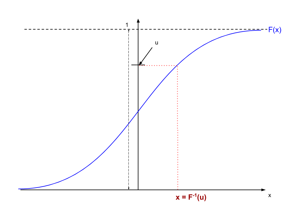
- Invert the mathematical function for the CDF of $X$ at the value of $u$, $$x = F^{-1}(u).\nonumber$$ Then $x\sim F$.
- Come up with a way to simulate draws from the Uniform distribution.
- Have the ability to invert the CDF of the random variable you want to simulate. The Inversion task requires a formula (if one exists) or a numerical algorithms for computing functions and inverses of functions. The procedures for all common random variable CDFs have been known for decades and are built into Ox and any other statistical package, mathematics library, etc. We will rely on these routines and not discuss how they work. The key to a Uniform RNG is not to just to produce numbers between 0 and 1 that are equally likely, but also to produce sequences of numbers that look like independent draws from the uniform distribution. To assess this aspect of RNGs we need to understand the notion of autocorrelation.
- Given $X\sim F(x)$.
- Set $r=1$ (the first observation). Draw $u^r \ {\buildrel pseudo \over \sim}\ U(0,1)$. This is one pseudo-random replication of a IID uniform random variable.
- Find the value $x^r$ such that $F(x^r)=u^r$.
- That is, compute $x^r = F^{-1}(u^r)$. Based on the theorem above, $x^r$ is a simulated draw from the distribution $F(x)$: $$x^r \ {\buildrel pseudo \over \sim}\ F(x).\nonumber$$ The inverse of the cdf can be computed either as a closed form for the inverse of the cdf or it can be computed $x^i$ numerically using computer algorithms.
- Increment $r$ and repeat. A pseudo IID sample is then $X_{r=1,\dots,R} \ {\buildrel pseudo \over \sim}\ F(x)$.
- Pseudo-Random Numbers in Ox
Function Pseudo-Random Operation ------------------------------------------------------------- ranu(r,c) generate a r×c matrix of uniform pseudo-random numbers rann(r,c) generate matrix of standard normal distributed pseudo-random numbers ranseed(iseed) set and get seed, or choose random number generator (depending on iseed)29-rand.ox 1: #include "oxstd.h" 2: main() { 3: println(ranu(3,2)); 4: println(ranu(1,4)); 5: ranseed(-1); 6: println(ranu(2,2)); 7: ranseed(33); 8: println(ranu(2,2)); 9: }- Output
      0.56444      0.76994
      0.41641      0.15881
     0.098209      0.37477

      0.56912      0.44078      0.47337      0.71055

      0.56444      0.76994
      0.41641      0.15881
The first uniform random number generated by an ox program is always 0.56444, unless your program has set the seed with
NR 7.0
There is nothing random about the operation of a computer, except to the extent that cosmic rays and products of truly random radioactive decay might scramble memory. Yet computers appear to generate random events. Doesn't your phone shuffle your playlist? Yet, there is nothing random about the operation of the microprocessor on the phone. If your computer/phone/tablet starts to act in a truly random fashion it is time to get a new one.
In the modern world we are surrounded by simulated randomness. One of the most important uses of computers in econometrics is to simulate randomness. What is meant by this is something quite specific. What is really important to simulate is independent sampling from a distribution. That is, computer algorithms have been developed to fake IID sampling.
Exhibit 45. Continuous and Discrete CDFs
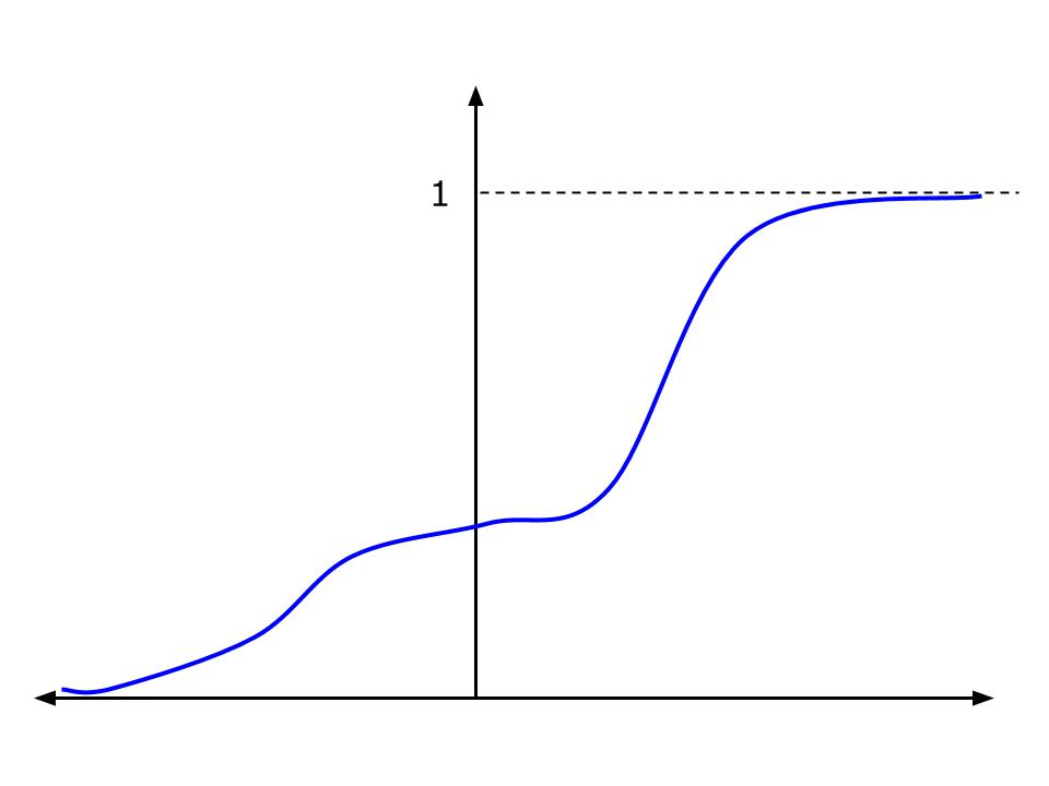
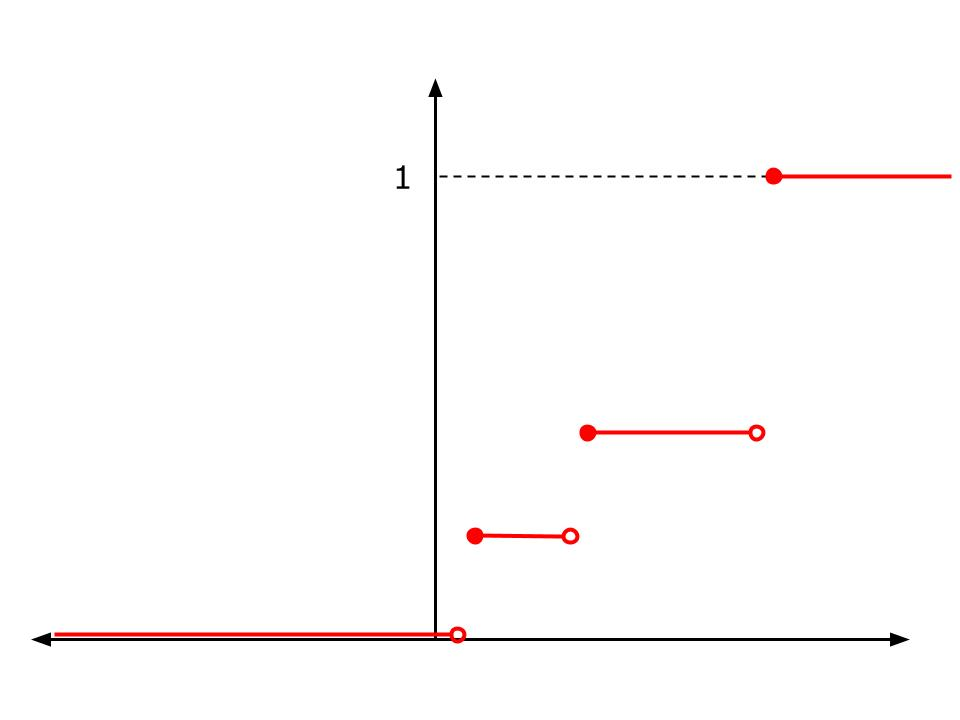
Right: The CDF of a discrete random variable. The jump points are values the random variable takes on. The size of the jump is the probability (pdf) of that value.
Definition 4. Marginal Distributions of Random Variables
Exhibit 46. The Uniform PDF and CDF
Definition 5. The Standard and General Normal Distributions
We write $Z\sim {\cal N}(0,1)$ to mean:
Exhibit 47. Bell Curves
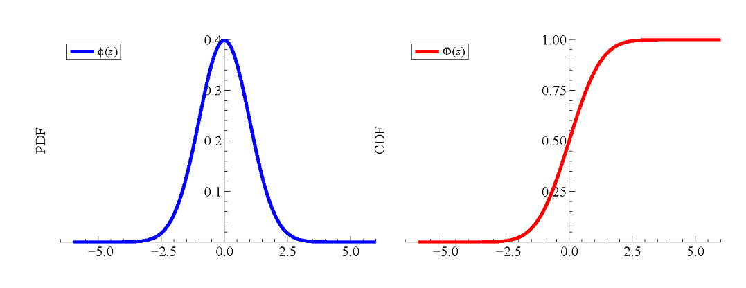
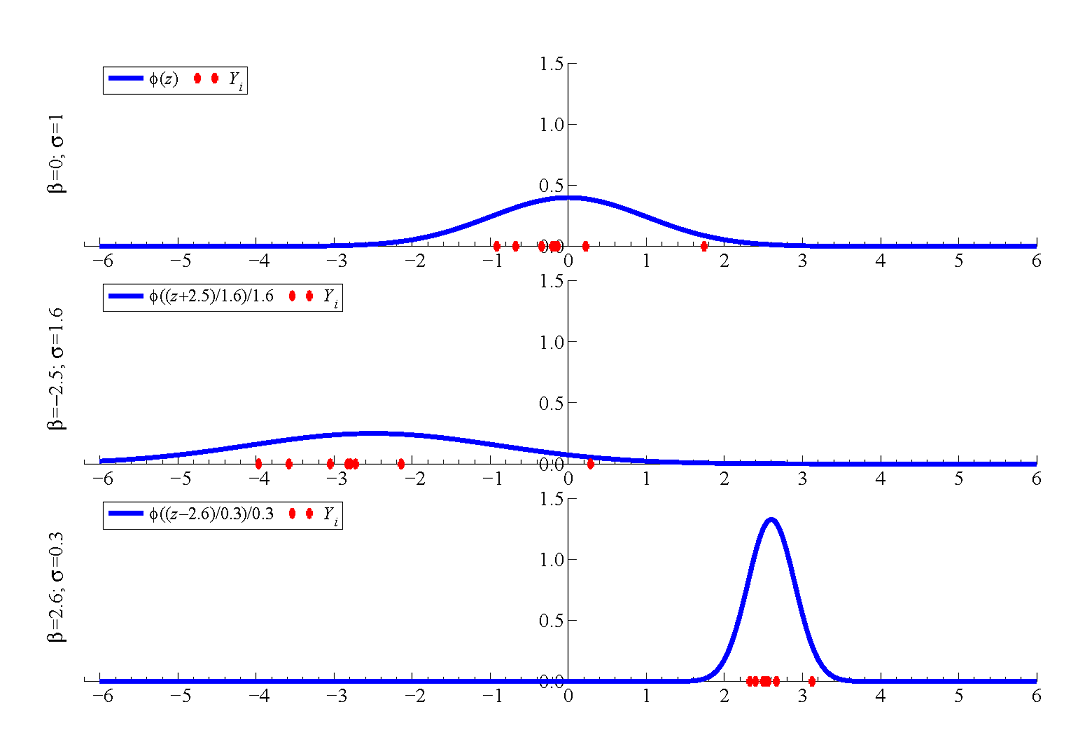
Right: Three Different Normal Densities with different means and variances.
Definition 6. Pseudo-Random Number Generator (pRNG)
Algorithm 21. Generating a random draw from (almost) any CDF
Given a CDF $F(x)$ and its mathematical inverse function, $F^{-1}(u)$.
Below is a CDF of a random variable $X$ that looks like the cumulative normal cdf, but does not need to be that function. Like all CDFs, it takes on values between 0 and 1 along the vertical axis. The Uniform random number generator produces a number between 0 and 1 with equal probability everywhere in that range. The realized value is marked $u$, around 0.75 in this case. This value is inverted to find the value of $x$ for which $F(x) = u$. If we repeat this procedure over-and-over again and the Uniform random number generator is working properly the histogram of values of $x$ will pile up like the pdf $f(x)$. As the number of replications went to infinity the histogram would converge to $f(x)$ exactly.
Exhibit 48. Inverting the CDF to Simulate a Random Experiment
Algorithm 22. Simulate an IID Sample (continuous)
Table 13. Basic Pseudo-Random Functions in Ox
oxprob package (so you have to #include oxprob.oxh. This simple program produces the output below:
ranseed() first. In fact, the first 10 draws are exactly what you see in the first two matrices. Then note that the next line sends -1 to ranseed(), which resets the seed to its initial value. Thus the next call to ranu() returns the first four numbers again.