C<sup>4</sup>E: Computation For Economists

Newton-Raphson and Broyden

NR 9.4, 9.6; Judd II.5.5

To Solve Non-Linear: Solve Linear Over and Over

root of the system

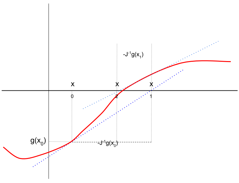
Newton-Raphson is a centuries-old algorithm to find the root of a non-linear system which uses the Jacobian of the system. It "pretends" that the system is linear to from one guess of the root to another. A linear system has a constant Jacobian, so each time the algorithm iterates it recomputes the Jacobian and solves another linear system. To understand Newton-Raphson, start with the situation when the system really is linear. That means we can write $g(x)$ as: $$g(x) = Ax+b,\nonumber$$ where $A$ is a square matrix and $b$ is a $n\times 1$ vector of constants. Of course, if a linear system has a solution it is closed-form: $x^\star = -A^{-1}b$. That is, if we can compute $A^{-1}$, then we can find the $x^\star$ that is the unique root of the system.

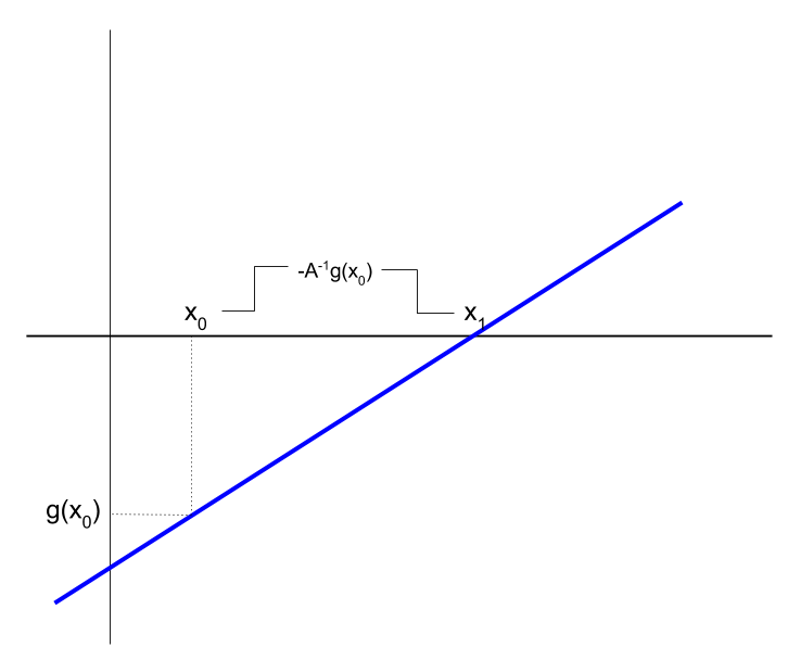
Given $A^{-1}$ is available, an iterative or sequential solution is not needed to solve a linear system, but we can think of it like an iteration solution which might help to see how non-linear methods build on linear ones. That is, suppose we started at a guess $x_0$. The value of the system at that point is $g(x_0) = Ax_0 + b$. If we wanted to get to $x^\star$ from there we could say: $$x^\star = x_1 \equiv x_0 - A^{-1}(b+Ax_0) = x_0 - A^{-1}g(x_0).\nonumber$$ In other words, we find the root by subtracting a vector from the initial guess $x_0$. We take a step from $x_0$ to get a new value $x_1$. The size of the step is such that we wipe out the difference $g(x_0)$. Reminder: It is typically inefficient to actually compute $A^{-1}$. Instead, solve linear system $$A s = -g\nonumber$$ to determine a step: $x_1 = x_0 + s.$

Algorithm 12. Newton-Raphson Iteration

Given $g(x)$, and $x_0\in \Re^n$. Attempt to find a solution to

Set $t=0$. Compute $g_t = g(x_t)$.
Strong convergence: $\|g_t\| \mathop{=_{\epsilon_1}} 0$, then . (Here $\mathop{=_{\epsilon_1}}$ means equal with tolerance $\epsilon_1$ that Ox's fuzzy-equal comparison functions implements.)
→ Compute the Jacobian at the new values, $J_t = Jg(x_t)$.

Solve $J_ts_t = -g_t$ for $s_t$.

Set $x_{t+1} = x_t + s_t$.

Lack of convergence: if $J_t$ is (nearly) singular or $x_{t+1}\mathop{=_{\epsilon_2}} x_t$, then

Increment $t$ and go back to step →.

quadratic

It is not always feasible to program analytic $J$. If numeric $J$ is used, then the number of evaluations required for each step is $1+2n$. If the cost of calculating $g(x)$ is linear in $n$ then computational cost of each step is quadratic in the size of the system $n$.

Although Newton-Raphson converges quickly there is no guarantee that any of the Newton-Raphson step will be an improvement or that it will ever converge. The behaviour depends on $Jg$, which may be badly behaved far from a root. May be near singular and steps may diverge. An alternative discussed next is to use information from past evaluations to build up an approximation to $J_t$ without computing it. Finally, there is no systematic way to use Newton-Raphson to find all roots. Methods to attempt that harder task are not discussed here.

Judd page 153, eq (5.2.4)

Broyden (Approximate Jacobian).

NR 9.7, page 389

Algorithm 13. Broyden's Method

Given $g(x)$, and $x_0\in \Re^n$.

Initialize. Set $t=0$; compute $g_0 = g(x_0)$; Set $J_0$ to a (well-conditioned) $n\times n$ matrix. Typically, $J_0 = I$.
Check for strong convergence: if $\|g_t\|\mathop{=_{\epsilon_1}}0$ then .
Otherwise, solve $J_t s_t = g_t$ for $s_t$. Set $x_{t+1} = x_t - s_t$. Check for non-convergence: If $\|x_{t+1}-x_t\| \mathop{=_{\epsilon_2}}0$ possibly reset $J_t$ to $J_0$ or simply .
Update Jacobian. Compute $g_{t+1}=g(x_{t+1})$ Let $y=g_{t+1}-g_t$. Then $${J_{t+1} = J_t +{(y-J_t s_t)s_t^T\over \|s_t\|}.}\nonumber$$
Increment $t$ and return to 1.

The key to the algorithm is the updating formula for the Jacobian. It is a good formula because it can be shown that it gets closer and closer to the actual Jacobian as the iteration proceeds and the process progresses. It is more robust to the initial value $x_0$ than Newton-Raphson, but still there is no guarantee of convergence. If convergence fails, restart at final values, which sometimes allows for further progress.

Non-linear Systems in Ox

solvenle

#import "solvenle";

    SolveNLE(func, ax, ...)

        Argument        Explanation
        ------------------------------------------------------------------------------------
        func            function evaluating the nonlinear system in the form below
        ax		        address of n x 1 matrix with starting values x0
                        final coefficients are placed in this location x*
         ...            Several optional arguments to control the algorithm (see below)

SolvenLE

function

SolveNLE

&

SolveNLE

    SolveNLE(func, ax, iMode, fJac )

        Argument     Explanation
        ------------------------------------------------------------------------------------
        iMode        integer code to choose the algorithm
                     -1 (default)	
                         Newton-Raphson with numerical Jacobian if n < 80
                         modified Newton-Raphson for n >= 80
                      0	Newton-Raphson using ANALYTIC Jacobian computed by fJac()
                      1	Newton-Raphson using numerical Jacobian computed by SolveNLE()
                      2	Broyden's method
                      3	modified Newton-Raphson that avoids storing nxn Jacobian matrix

        fJac          If iMode==0 then fJac() has to return the Jacobian matrix
                      This would be useful if you have coded the analytic form of the Jacobian
                      and computing numerical Jacobians is expensive.

The supplied func argument should have the following format:

	func(ag, x)

        Argument        Explanation
        ------------------------------------------------------------------------------------
        ag              address for where to put the n x 1 vector value of g(x)
        x               n x 1 vector of x values

	Returns
        1: successful,
        0: function evaluation failed

Example

Code

25-nle-example.ox
 1:    #include "oxstd.h"
 2:    #import "solvenle"
 3:    myg(fv,x) {
 4:        if (x<=0) return FALSE;
 5:        fv[0] = log(x) + x^2;
 6:    	println("%13.8f",x~fv[0]);
 7:        return TRUE;
 8:        }
 9:    main(){
10:        decl x = <1.0>,ccode;
11:        ccode = SolveNLE(myg,&x);
12:        println("Convergence code: ",ccode,"\nSolution: ",x);
13:        }

Output:

Convergence code: 0
Solution:
      0.65292

Exercises

Modify 26-poly-roots.ox to find all the roots of the polynomial of $g(x) = 1+x-2x^2-x^3+0.5x^4-0.1x^5$. Then code a function in the form needed by SolveNLE() that uses polyeval() to evaluate the polynomial. Call SolveNLE() and see if it converges to one of the real roots and whether it converges to different roots based on initial values or choice of Newton-Raphson or Broyden. After experimenting, write a program that starts SolveNLE() at different values that converge to different roots.
Consider a 2x2 system of the form: $g(x) = \l(\matrix{g_0(x)\cr g_1(x)}\r)$ $$\eqalign{ g_0(x) &= \log(x_0) - x_1^2\cr g_1(x) &= \sin(x_1) - \cos(x_0)\cr }\nonumber$$
1. Write a function called sys_internal(x) that expects a 2x1 vector and returns $g(x).$ Test your code by sending the vector $\l(\matrix{1\cr 1}\r)$ to sys_internal() and printing the output. You should get g():
```
      -1.0000
      0.30117
```
2. Write a new function named sys() that follows the format required by SolveNLE and is a "wrapper" around your simpler sys_internal() function:
```
sys(ag,x)
```
  It returns either 0 if $x_0<0$, otherwise it calls sys_internal() and returns 1. Verify your sys computes the correct value for <1;1> and returns 1.
3. Use SolveNLE to solve for a root of the system. Check the convergence code. Try different starting values to see if it finds more than one root. Start at an undefined value (say $x_0=-1$) and see what happens.
On the $x_0$-$x_1$ plane the intersection of a line and a circle is the solution of a non-linear system. The particular system is of the form $$g(x) = \left(\matrix{g_0 \cr g_1 }\right) = \left(\matrix{ x_0+x_1 - v \cr x^2_0 + x^2_1 - 9 \cr}\right).$$ The parameter $v$ should be stored as global variable. Set it to $v=3.$ You should be able to see there are two solutions at $(0,3)$ and $(3,0)$. Further, the analytic Jacobian is easily computed as $$Jg(x) =\left(\matrix{ 1 & 1 \cr 2x_0 & 2x_1 \cr}\right)$$
1. Solve this problem numerically using SolveNLE() and Broyden's method following examples already done. Start with use of a numerical Jacobian.
2. Write your main code to start at values near the two solutions and see if they converge to the closest one.
3. Code the analytic Jacobian and run Newton-Raphson with it.
4. If you increase $v$ from 3 the two roots move closer together until eventually they meet when the line is tangent to the circle. If you go past that point there is no solution. Experiment with changing $v$ to find the tangency and see what happens when no solution exists. Here is a loop that would make it easier to do this ... insert in your main code and adjust $v$. You might also confirm analytically the value of $v$ that results in a unique root and enter it to confirm.
```
while (TRUE) {
    scan("Enter v ","%g",&v);
    // reset your starting/ vector here
    SolveNLE( ...  );
    }
    
```

Newton-Raphson and Broyden

Exhibit 38. Linear System as an Iteration

Algorithm 12. Newton-Raphson Iteration

Exhibit 39. Newton-Raphson Iteration

Algorithm 13. Broyden's Method

Exercises