-
The
- Here are the primary functions for graphing data stored in vectors and matrices:
Function What It Does ---------------------------------------------------------------------------------------------- DrawXMatrix() plot multiple variables in a matrix against a row-vector of x values see also simpler Draw() & DrawX() DrawXYZ() plot 3-D contours or surfaces DrawZ() add a 3rd dimension to a XY plot DrawDensity() plot a histogram of data. - You can also add text, lines and shapes to a graph with these routines:
DrawLine() DrawSymbol() DrawText()
- Finally, you can adjust the axes and other aspects of plot with:
Again, other functions are available, but the ones listed above will handle basic cases.DrawAdjust() DrawAxis() DrawAxisAuto()
- Draw an Indifference Curve
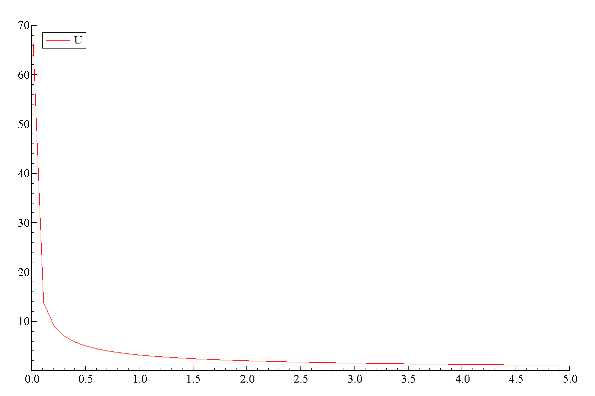
To illustrate how to useoxdraw, consider the task of plotting an indifference curve for the Cobb-Douglas utility function, $U(x_0,x_1) = x_0^\alpha x_1^{1-\alpha}$. An indifference curve is the set of bundles that give equal utility: $$\left\{\ (x_0,x_1):\ x_0^\alpha x_1^{1-\alpha} = {\bar u} \right\}.\nonumber$$ The curve is defined by the number ${\bar u}$. Any combination of $(x_0, x_1)$ that yield that utility is on the indifference curve (in the set). The curve on a graph is then a function of $x_0$ that gives the value of $x_1$ that pairs with it on the curve. So we have to solve the equation above for $x_1$: $$x_1\left(x_0;{\bar u},\alpha\right) = \left[ {\bar u}/x^\alpha \right]^{1\over 1-\alpha}.\nonumber$$ To draw an indifference curve, pick a value of $\alpha$, a level ${\bar u}$ and then many different values of $x_0$ to graph $x_1(x_0; {\bar u},\alpha\bigr)$.16-plot2.ox 1: #include
2: #include 3: 4: const decl alpha=0.4, 5: u0 = 2.1; 6: main() { 7: decl indiff, x0; 8: x0 = range(0.01,5,.1); 9: indiff = ( u0./x0.^alpha ).^(1/(1-alpha)); 10: DrawXMatrix(0, indiff,{"U="+sprint(u0)},x0,"x"); 11: SaveDrawWindow("icurve.pdf"); 12: } #include "oxdraw.oxh"(line 2). We will useDrawXMatrix()in this example. The code sets $\alpha = 0.4$ and ${\bar u} = 2$. Then it generates a range of values for $x_0 = $.01 .11 .21 .31 … 4.91. Notice thatrange()produces a row vector which is whatDrawXMatrixexpects. If you send it a column vector for $x_0$ it won't work properly. The program then creates the corresponding values of $x_1$ on the indifference curve, storing it inindiff, which will also be a row vector. Now we use the main graphics routine. It is easier to explain the arguments if we split them across lines:DrawXMatrix( 0, // Area to draw in (0 = top left graph) indiff, // matrix to draw on the y-axis {"U="+sprint(u0)}, // label(s) for each row of data x0, // values for the x-axis "x" // label for x );DrawXMatrix()is0. That means this command will affect the first graph area. You can create multiple graphs to be viewed together by drawing in areas 1, 2, 3, etc. The next two arguments are the matrix to draw followed by an array of labels to give the rows. Here we want the label to show the level of utility, so it will showU=2.1
, then the x vector followed by its own label. At this point the graph exists internally in Ox but it won't be produced untilSaveDrawWindow()is called. That means that subsequentoxdrawfunctions could add other things to the graph or specialize it in other ways.The argument sent to
SaveDrawWindowis the name of the file. Since the extension is.pdf
the file is saved as PDF. The other formats that Ox Console will save to are probably not useful to you. This is one of the limitations of the free version of Ox. The professional version allows you to view graphs interactively and to save them to image formats by copying it the clipboard.Exhibit 24. An Indifference Curve

Suppose we wanted to view not just the line but the evaluated points at each pair of points as well. We can do that by adding one of the optional arguments to
DrawXMatrixinstead of using the default value. Namely:DrawXMatrix(0, indiff, {"U="+sprint(u0)}, x0, "x", 2 ); ↑DrawXMatrix(0, indiff, {"U="+sprint(u0)}, x0, "x", ST_LINESYMBOLS); ↑oxdraw. It is not easy compared to a menu-driven system, but it is very easy to make sophisticated graphs within a program.- Three-Dimensional Graphs
Sorry ... not done - Finally, you can adjust the axes and other aspects of plot with:
oxdraw module is powerful but not particularly easy to use. And the documentation does not make it easy to get started. Because Ox can save data to spreadsheet files and Stata .dta files, it is often easiest just to produce graphs using other packages. However, if your project is designed to be self-contained it might be more useful to include internally generated graphs.
This section builds on efforts by me and past students to using graphs in Ox. In particular, only features available in Ox Console of general use are covered. It does not discuss specialized graphs or features requiring OxMetrics. http://www.doornik.com/ox/oxdraw.html or clicking on "Graphics reference" in the Ox documentation provides complete description of the package.
Exercises
16-plot2.ox so that multiple indifference curves are produced. To do this change u0 from a scalar to a column vector. (Getting the labels requires changing the third argument of DrawXMatrix.)